|
Bruno Contreras-Moreira (1) and Pablo Vinuesa (2)
1. EstaciĂłn Experimental de Aula Dei-CSIC
2. Centro de Ciencias GenĂłmicas, Universidad Nacional AutĂłnoma de MĂ©xico
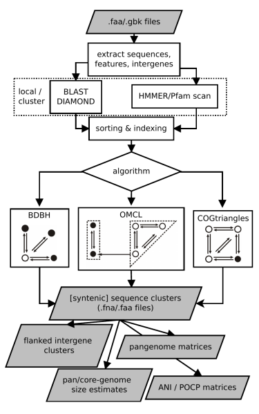
This document describes the software GET_HOMOLOGUES and provides a few examples on how to install and use it. The source code and issue manager can be found at https://github.com/eead-csic-compbio/get_homologues. get_homologues is mainly written in the Perl programming language and includes several algorithms designed for three main tasks:
While the program was mainly developed for the study of bacterial genomes in GenBank format, it can also be applied to eukaryotic sets of sequences, although in this case the meaning of terms such as core- or pan-genome might change, and intergenic regions might be longer.
The twin
manual_get_homologues-est.pdf
file describes the specific options of get_homologues-est,
designed and tested for the task of clustering transcripts and, more generally, DNA-sequences of strains of the same species.
The output files of GET_HOMOLOGUES can be used to drive phylogenomics and population genetics analyses with the kin pipeline GET_PHYLOMARKERS.
get_homologues.pl is a Perl5 program bundled with a few binary files. The software has been tested on 64-bit Linux boxes, and on Intel MacOSX systems. Therefore, a Perl5 interpreter is needed to run this software, which is usually installed by default on these operating systems. In addition, the package includes a few extra scripts which can be useful for downloading GenBank files and for the analysis of the results.
In order to install and test this software please follow these steps:
$ tar xvfz get_homologues_X.Y.tgz
$ cd get_homologues_X.Y
$ perl install.pl
$ ./get_homologues.pl -v which will tell exactly which features are available.
get_homologues.pl, with the included sample input folder sample_buch_fasta
by means of the instruction:
$ ./get_homologues.pl -d sample_buch_fasta .
You should get an output similar to the contents of file sample_output.txt.
$PATH environment variable to include get_homologues.pl.
Please copy the following lines to the .bash_profile or
.bashrc files, found in your home directory, replacing [INSTALL_PATH] by the full path of the installation folder:
export GETHOMS=[INSTALL_PATH]/get_homologues_X.Y
export PATH=${GETHOMS}/:${PATH}
This change will be effective in a new terminal or after running: $ source ~/.bash_profile
If you prefer a copy of the software that can be updated in the future you can get it from the GitHub repository with:
$ git clone https://github.com/eead-csic-compbio/get_homologues.git
$ perl install.pl
$ cd get_homologues
$ git pull
Finally, you can also install the software from bioconda as follows:
$ conda activate bioconda
$ conda create -n get_homologues -c conda-forge -c bioconda get_homologues
$ conda activate get_homologues

# only if you want to install Pfam or SwissProt db
$ perl install.pl
See section 2.3 to learn how to configure the software to run on a HPC environment.
The rest of this section might be safely skipped if installation went fine, it was written to help solve installation problems.
A few Perl core modules are required by the get_homologues.pl script, which should be already installed on your system: Cwd, FindBin, File::Basename, File::Spec, File::Temp, FileHandle, List::Util, Getopt::Std, Benchmark and Storable.
In addition, the Bio::Seq, Bio::SeqIO, Bio::Graphics and Bio::SeqFeature::Generic modules from the Bioperl collection, and module Parallel::ForkManager are also required, and have been included in the get_homologues bundle for your convenience.
Should this version of BioPerl fail in your system (as diagnosed by install.pl)
it might be necessary to install it from scratch.
However, before trying to download it, you might want to check whether
it is already living on your system, by typing on the terminal:
$ perl -MBio::Root::Version -e 'print $Bio::Root::Version::VERSION'
If you get a message Can't locate Bio/Root/Version... then you need to actually install it, which
can sometimes become troublesome due to failed dependencies. For this reason usually the easiest way of
installing it, provided that you have root privileges,
it is to use the software manager of your Linux distribution (such as synaptic/apt-get
in Ubuntu, yum in Fedora or YaST in openSUSE). If you prefer the terminal please use the
cpan program with administrator privileges (sudo in Ubuntu):
$ cpan -i C/CJ/CJFIELDS/BioPerl-1.6.1.tar.gz
This form should be also valid:
$ perl -MCPAN -e 'install C/CJ/CJFIELDS/BioPerl-1.6.1.tar.gz'
Please check this tutorial
if you need further help.
The accompanying script download_genomes_ncbi.pl imports File::Fetch, which
should be bundled by default as well. In case it is missing on your Fedora systems, it can be installed
as root with: $ yum install perl-File-Fetch
The Perl script install.pl, already mentioned in section 2, checks whether the included precompiled binaries for COGtriangles, hmmer, MCL and BLAST are in place and ready to be used by get_homologues. However, if any of these binaries fails to work in your system, perhaps due a different architecture or due to missing libraries, it will be necessary to obtain an appropriate version for your system or to compile them with your own compiler.
In order to compile MCL the GNU gcc compiler is required, although it should most certainly already be
installed on your system. If not, you might install it by any of the alternatives listed in section 2.1.
For instance, in Ubuntu this works well: $ sudo apt-get install gcc . The compilation steps are
as follows:
$ cd bin/mcl-14-137;
$ ./configure`;
$ make
To compile COGtriangles the GNU g++ compiler is required. You should obtain it by any of the alternatives listed below:
$ yum -y install gcc-c++        # Redhat and derived distros

$ sudo apt-get -y install g++   # Ubuntu/Debian-based distros, and then cpan below
The compilation would then include several steps:
$cd bin/COGsoft;
$cd COGlse; make;
$cd ../COGmakehash;make;
$cd ../COGreadblast;make;
$cd ../COGtriangles;make
Regarding BLAST, get_homologues uses BLAST+ binaries, which
can be easily downloaded from the NCBI FTP
site.
The packed binaries are blastp and makeblastdb from version ncbi-blast-2.17.0+. If these do
not work in your machine or your prefer to use older BLAST versions, then it will be necessary to
edit file lib/phyTools.pm. First, environmental variable $ENV{'BLAST_PATH'} needs to be set to
the right path in your system (inside subroutine sub set_phyTools_env).
Variables $ENV{'EXE_BLASTP'} and $ENV{'EXE_FORMATDB'} also need to be changed to the appropriate
BLAST binaries, which are respectively blastall and formatdb.
It is possible and recommended to run get_homologues on a high-performance computing (HPC) cluster
invoking the program with option -m cluster.
For gridengine
environments (6.0u8, 6.2u4, 2011.11p1)
the script should work out of the box. For LSF
and
Slurm
settings a configuration step is required.
In these cases you would need to create a file named HPC.conf
in the same location as get_homologues.pl tayloring your queue configuration and paths.
Alternatively it is possible to create a configuration file anywhere in your filesystem,
with -m /path/custom/HPC.conf, which is useful for work for conda installs.
Check the sample configuration file at
sample.HPC.conf.
If your computer farm is managed by LSF,
you should create a file named HPC.conf modifiying the provided template sample.HPC.conf
and adding a full path if necessary:
# cluster/farm configuration file, edit as needed (use spaces or tabs)
# comment lines start with #
# PATH might be empty or set to a path/ ending with '/', example:
#PATH	/lsf/10.1/linux3.10-glibc2.17-x86_64/bin/
TYPE	lsf
SUBEXE	bsub
CHKEXE	bjobs
DELEXE	bkill
ERROR	EXIT
If your farm is managed by Slurm
instead,
the contents of the configuration file HPC.conf should be similar to this:
TYPE	slurm
SUBEXE	sbatch
CHKEXE	squeue
DELEXE	scancel
ERROR	F
For backwards compatibility, we provide here instructions on how to set up your own Grid Engine cluster.
### Debian 11 install (updated 08112021)
### (explained in Spanish at
### https://bioinfoperl.blogspot.com/2021/10/howto-install-grid-engine-on-multi-core-box-debian.html.html)

   # this also creates user sgeadmin
   sudo apt install gridengine-master gridengine-qmon gridengine-exec

   # edit /etc/hosts
   127.0.0.1 localhost.localdomain localhost
   127.0.1.1 master master
   121.xxx.yyy.zzz myhost

   # give yourself provileges
   sudo -u sgeadmin qconf -am myuser

   # and to a userlist
   qconf -au myuser users

   # Add a submission host
   qconf -as myhost

   # Add an execution host, you will be prompted for information about the execution host
   qconf -ae

   # Add a new host group
   qconf -ahgrp @allhosts

   # Add the exec host to the @allhosts list
   qconf -aattr hostgroup hostlist myhost @allhosts

   # Add and configure queue, set the slots matching your CPU/cores
   qconf -aq all.q

   # Add the host group to the queue
   qconf -aattr queue hostlist @allhosts  all.q

   # Make sure there is a slot allocated to the execd
   qconf -aattr queue slots "[myhost=1]" all.q


### Ubuntu install from SourceForge (updated 08112021)

# 1) go to  https://sourceforge.net/projects/gridengine/files/SGE/releases/8.1.9 ,
# create user 'sgeadmin' and download the latest binary packages
# (Debian-like here) matching your architecture (amd64 here):

wget -c https://sourceforge.net/projects/gridengine/files/SGE/releases/8.1.9/sge-common_8.1.9_all.deb/download
wget -c https://sourceforge.net/projects/gridengine/files/SGE/releases/8.1.9/sge_8.1.9_amd64.deb/download
wget -c https://sourceforge.net/projects/gridengine/files/SGE/releases/8.1.9/sge-dbg_8.1.9_amd64.deb/download

sudo useradd sgeadmin
sudo dpkg -i sge-common_8.1.9_all.deb
sudo dpkg -i sge_8.1.9_amd64.deb
sudo dpkg -i sge-dbg_8.1.9_amd64.deb
sudo apt-get install -f

# 2) set hostname to anything but localhost by editing /etc/hosts so that
# the first line is something like this (localhost or 127.0.x.x IPs not valid):
# 172.1.1.1   yourhost

# 3) install Grid Engine server with defaults except cluster name ('yourhost')
# and admin user name ('sgeadmin'):
sudo su
cd /opt/sge/
chown -R sgeadmin sge
chgrp -R sgeadmin sge
./install_qmaster

# 4) install Grid Engine client with all defaults:
./install_execd
exit

# 5) check the path to your sge binaries, which can be 'lx-amd64'
ls /opt/sge/bin

# 6) Set relevant environment variables in /etc/bash.bashrc [can also be named /etc/basrhc]
# or alternatively in ~/.bashrc for a given user
export SGE_ROOT=/opt/sge
export PATH=$PATH:"$SGE_ROOT/bin/lx-amd64"

# 7) Optionally configure default all.q queue:
qconf -mq all.q

# 8) Add your host to list of admitted hosts:
qconf -as yourhost
It is possible to invoke Pfam domain scanning from get_homologues. This option
requires the bundled binary hmmscan, which is part of the HMMER3
package,
whose path is set in file lib/phyTools.pm (variable $ENV{'EXE_HMMPFAM'}).
Should this binary not work in your system, a fresh install might be the solution, say in /your/path/hmmer-3.1b2/.
In this case you'll have to edit file lib/phyTools.pm and modify the relevant:
if( ! defined($ENV{'EXE_HMMPFAM'}) )
{
	$ENV{'EXE_HMMPFAM'} = '/your/path/hmmer-3.1b2/src/hmmscan --noali --acc --cut_ga ';
}
The Pfam HMM library is also required and the install.pl script should take care of it.
However, you can manually download it from the appropriate
Pfam FTP site.
This file needs to be decompressed, either in the default db folder or in any other location,
and then it should be formatted with the program hmmpress, which is also part of the
HMMER3 package. A valid command sequence could be:
$ cd db;
$ wget https://ftp.ebi.ac.uk/pub/databases/Pfam/current_release/Pfam-A.hmm.gz .;
$ gunzip Pfam-A.hmm.gz;
$ /your/path/hmmer-3.1b2/src/hmmpress Pfam-A.hmm
Finally, you'll need to edit file lib/phyTools.pm and modify the relevant line to:
if( ! defined($ENV{"PFAMDB"}) ){ $ENV{"PFAMDB"} = "db/Pfam-A.hmm"; }
In order to reduce the memory footprint of get_homologues it is possible to take advantage of the
Berkeley_DB
database engine, which requires Perl core module
DB_File, which should be installed on all major Linux distributions.
If DB_File is not found within a conda environment you might have to run conda deactivate before.
Should manual installation be required, this can be done as follows:
$ yum -y install libdb-devel         # Redhat and derived distros

$ sudo apt-get -y install libdb-dev  # Ubuntu/Debian-based distros, and then cpan below

$ cpan -i DB_File                    # requires administrator privileges (sudo)
Similarly, in order to take full advantage of the accompanying script parse_pangenome_matrix.pl,
particularly for option -p, the installation of module GD
is recommended.
An easy way to install them, provided that you have administrator privileges,
is with help from the software manager of your Linux distribution (such as synaptic/apt-get
in Ubuntu, yum in Fedora or YaST in openSUSE).
This can usually be done on the terminal as well, in different forms:
$ sudo apt-get -y install libgd-gd2-perl  # Ubuntu/Debian-based distros

$ yum -y install perl-GD                  # Redhat and derived distros

$ zypper --assume-yes install perl-GD     # SuSE

$ cpan -i GD                              # will require administrator privileges (sudo)

$ perl -MCPAN -e 'install GD'             # will require administrator privileges (sudo)
The installation of perl-GD on macOSX systems is known to be troublesome.
The accompanying scripts compare_clusters.pl, plot_pancore_matrix.pl, parse_pangenome_matrix.pl,
plot_matrix_heatmap.sh, hcluster_pangenome_matrix.sh require the installation of the statistical software
R,
which usually is listed by software managers in all major Linux distributions.
In some cases (some SuSE versions
and
some Redhat-like distros)
it will be necessary to add a repository to your package manager.
R can be installed from the terminal:
$ sudo apt-get -y install r-base r-base-dev      # Ubuntu/Debian-based distros

$ yum -y install R                               # RedHat and derived distros

$ zypper --assume-yes R-patched R-patched-devel  # Suse
Please visit CRAN
to download and install R on macOSX systems, which is straightforward.
In addition to R itself, plot_matrix_heatmap.sh and hcluster_pangenome_matrix.sh require some R packages to run, which can be easily installed from the R command line with:
> install.packages(c("ape", "gplots", "cluster", "dendextend", "factoextra"), dependencies=TRUE)
The script compare_clusters.pl might require the installation of program PARS from the
PHYLIP suite, which should be already bundled
with your copy of get_homologues.
Finally, download_genomes_ncbi.pl might require wget in order to download WGS genomes,
but should be installed on most systems.
This section describes the available options for the get_homologues software.
The input required to run get_homologues can be of two types:
| 1 | A single file with amino acid sequences in FASTA format,
in which headers include a taxon name between square brackets, including at least two words
and a first capital letter, as shown in the example:
>protein 123 [Species 1] MANILLLDNIDSFTYNLVEQLRNQKNNVLVYRNTVSIDIIFNSLKKLTHPILMLSPGPSLPKHAGCMLDL PEKFVINSYFEKMIMSVRNNCDRVCGFQFHPESILTTHGDQILEKIIHWASLKYITNKKQ >gi|10923402| [Species 2] IKKVKGDIPIVGICLGHQAIVEAYGGIIGYAGEIFHGKASLIRHDGLEMFEGVPQPLPVARYHSLICNKI PEKFVINSYFEKMIMSVRNNCDRVCGFQFHPESILTTHGDQILEKIIHWASLKYITNKKQ ... |
| 2 | A directory or folder containing several files in either FASTA format (extensions '.faa' or '.fasta', containing amino acid sequences) or GenBank files (extension '.gbk', one file per organism). The advantage of this option is that new files can be added to the input folder in the future and previous calculations will be conserved. This might be useful to study a group of organisms for which a few genomes are available, and then keep adding new genomes as they become available. This directory can actually contain a mixture of FASTA and GenBank files. |
The GenBank format is routinely used to describe genomic sequences, usually taking one file per chromosome or genomic contig. Each file contains a reference DNA genomic sequence plus a collection of genes and their products, making it possible to extract simultaneously the sequence of every ORF and its corresponding protein products.
GenBank files are the recommended input format for bacterial sequences, as they permit the compilation of DNA and protein sequences clusters, which might have different applications.
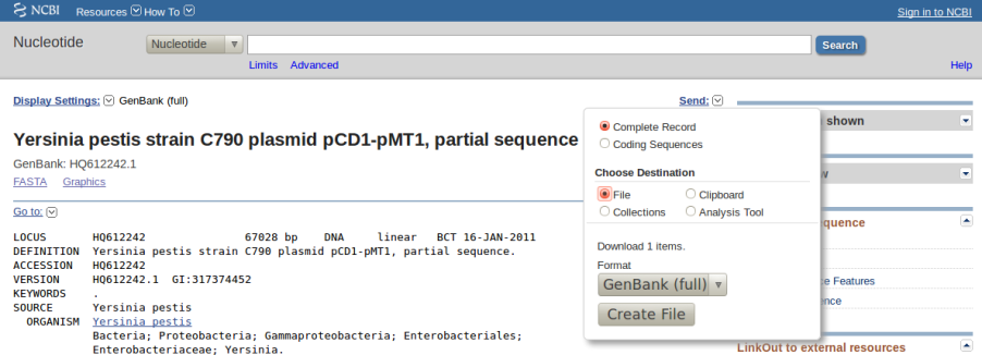
There are many ways to obtain GenBank files, starting by manual browsing and downloading from the NCBI site, keeping in mind that full files, which include the reference nucleotide sequences, should be downloaded. In fact, get_homologues.pl will fail to parse any ORF in summary GenBank files.
|
|
Often users take custom-made GenBank files, resulting from in-house genome assemblies, to be analysed.
In most cases genes from such files don't have GenBank identifiers assigned yet, and so we recommend
adding the field locus_tag to each CDS feature so that parsed sequences can be properly identified.
For their use with get_homologues, GenBank files for the same species (for example, from the main chromosome and from a couple of plasmids) must be concatenated. For instance, the genomic sequences of Rhizobium etli CFN 42 comprise <1013>>http://www.ncbi.nlm.nih.gov/genome?Db=genome&term=rhizobiumwhich can be concatenated into a single _Rhizobium_etli_CFN42.gbk file.
In order to assist in this task this software package includes the accompanying script download_genomes_ncbi.pl. We will explain its use by fetching some of the Yersinia pestis genomic sequences used in a 2010 paper by Morelli et al:
Group   Name         Accession Number    Status
0.PE2   Pestoides F  NC_009381           Completed Sanger genome
0.PE3   Angola       NC_010159           Completed Sanger genome
0.PE4   91001        NC_005810           Completed Sanger genome
0.ANT2  B42003004    NZ_AAYU00000000     Draft Sanger genome
1.ANT1  UG05-0454    NZ_AAYR00000000     Draft Sanger genome (12.3X coverage)
1.ANT1  Antiqua      NC_008150           Completed Sanger genome
1.IN3   E1979001     NZ_AAYV00000000     Draft Sanger genome
1.ORI1  CA88-4125    NZ_ABCD00000000     Draft Sanger genome
1.ORI1  FV-1         NZ_AAUB00000000     Draft Sanger genome
1.ORI1  CO92         NC_003143           Completed Sanger genome
1.ORI2  F1991016     NZ_ABAT00000000     Draft Sanger genome
1.ORI3  IP674        ERA000177           Draft 454 genome (82X coverage)
1.ORI3  IP275        NZ_AAOS00000000     Draft Sanger genome (7.6X coverage)
1.ORI3  MG05-1020    NZ_AAYS00000000     Draft Sanger genome (12.1X coverage)
2.ANT1  Nepal516     NZ_ACNQ00000000     Draft Sanger genome
2.MED1  KIM          NC_004088           Completed Sanger genome
2.MED2  K1973002     NZ_AAYT00000000     Draft Sanger genome
In order to use download_genomes_ncbi.pl is is necessary to feed it a text file listing which
genomes are to be downloaded. The next examples show the exact format required,
as does the bundled file sample_genome_list.txt.
First, it can be seen that completed genomes have NC accession numbers, and
can be added to the list as follows:
NC_010159 Yersinia_pestis_AngolaOther annotated genomes can be added using their assembly code, as in this example: can be added to the list as follows:
GCA_000016445.1_ASM1644v1 Yersinia_pestis_Pestoides_FFinally, draft WGS genomes, which can be browsed at
AAYU01 Yersinia_pestis_B42003004
Finally, the genome_list.txt file will look as this:
NC_010159                  Yersinia_pestis_Angola
GCA_000016445.1_ASM1644v1  Yersinia_pestis_Pestoides_F
AAYU01                     Yersinia_pestis_B42003004
Note that only the first two columns (separated by blanks) are read in, and that lines can be commented out by adding a '#' as the first character.
Now we can run the following terminal command to fetch these genomes:
$ ./download_genomes_ncbi.pl genome_list.txt
which will put several _Yersinia_pestis_*.gbk files in the current directory, which are now
ready to be used by get_homologues.
Due to the complexity of eukaryotic genomes, which are split in many chromosomes and contigs and usually contain complex gene models, the preferred format taken by get_homologues for their sequences is FASTA.
While eukaryotic GenBank files can be fed in, during development we have not tested nor benchmarked the compilation of clusters of nucleotide eukaryotic sequences, which can be more error prone due to the inclusion of, for instance, introns and pseudogenes. Therefore we currently cannot recommend the use of eukaryotic GenBank input files.
Of course FASTA format can also be used for prokaryotic amino acid sequences, as in the case of the
example sample_buch_fasta folder, which contains protein sequences found in four Buchnera aphidicola genomes.
If your data are DNA coding sequences you can translate them to protein sequences for use with get_homologues, for instance by means of a Perl command in the terminal, with a little help from Bioperl 2.1. It is a long command, which is split in three chunks to fit in this page:
$ perl -MBio::Seq -lne 'if(/^(>.*)/){$h=$1}else{$fa{$h}.=$_} \
	END{ foreach $h (sort(keys(%fa))){ $fa{$h}=Bio::Seq->new(-seq=>$fa{$h})->translate()->seq(); \
	print "$h\n$fa{$h}\n" }}' your_CDS_file.fna
-v print version, credits and checks installation
-d directory with input FASTA files ( .faa / .fna ),           (overrides -i,
   GenBank files ( .gbk ), 1 per genome, or a subdirectory      use of pre-clustered sequences
   ( subdir.clusters / subdir_ ) with pre-clustered sequences   ignores -c, -g)
   ( .faa / .fna ); allows for new files to be added later;
   creates output folder named 'directory_homologues'
-i input amino acid FASTA file with [taxon names] in headers,  (required unless -d is set)
   creates output folder named 'file_homologues'

Optional parameters:
-o only run BLAST/Pfam searches and exit                       (useful to pre-compute searches)
-c report genome composition analysis                          (follows order in -I file if enforced,
                                                                ignores -r,-t,-e)
-R set random seed for genome composition analysis             (optional, requires -c, example -R 1234,
                                                                required for mixing -c with -c -a runs)
-m runmode [local|cluster|dryrun|/path/custom/HPC.conf]        (def: local, path overrides ./HPC.conf)
-n nb of threads for BLAST/HMMER/MCL in 'local' runmode        (default=2)
-I file with .faa/.gbk files in -d to be included              (takes all by default, requires -d)

Algorithms instead of default bidirectional best-hits (BDBH):
-G use COGtriangle algorithm (COGS, PubMed=20439257)           (requires 3+ genomes|taxa)
-M use orthoMCL algorithm (OMCL, PubMed=12952885)

Options that control sequence similarity searches:
-X use diamond instead of blastp                               (optional, set threads with -n)
-C min %coverage in BLAST pairwise alignments                  (range [1-100],default=75)
-E max E-value                                                 (default=1e-05,max=0.01)
-D require equal Pfam domain composition                       (best with -m cluster or -n threads)
   when defining similarity-based orthology
-S min %sequence identity in BLAST query/subj pairs            (range [1-100],default=1 [BDBH|OMCL])
-N min BLAST neighborhood correlation PubMed=18475320          (range [0,1],default=0 [BDBH|OMCL])
-b compile core-genome with minimum BLAST searches             (ignores -c [BDBH])

Options that control clustering:
-t report sequence clusters including at least t taxa          (default t=numberOfTaxa,
                                                                t=0 reports all clusters [OMCL|COGS])
-a report clusters of sequence features in GenBank files       (requires -d and .gbk files,
   instead of default 'CDS' GenBank features                    example -a 'tRNA,rRNA',
                                                                NOTE: uses blastn instead of blastp,
                                                                ignores -g,-D)
-g report clusters of intergenic sequences flanked by ORFs     (requires -d and .gbk files)
   in addition to default 'CDS' clusters
-f filter by %length difference within clusters                (range [1-100], by default sequence
                                                                length is not checked)
-r reference proteome .faa/.gbk file                           (by default takes file with
                                                                least sequences; with BDBH sets
                                                                first taxa to start adding genes)
-e exclude clusters with inparalogues                          (by default inparalogues are
                                                                included)
-x allow sequences in multiple COG clusters                    (by default sequences are allocated
                                                                to single clusters [COGS])
-F orthoMCL inflation value                                    (range [1-5], default=1.5 [OMCL])
-A calculate average identity of clustered sequences,          (optional, creates tab-separated matrix,
   by default uses blastp results but can use blastn with -a      recommended with -t 0 [OMCL|COGS])
-P compute % conserved proteins (POCP) & align fraction (AF),  (optional, creates tab-separated matrices,
   by default uses blastp results but can use blastn with -a      recommended with -t 0 [OMCL|COGS])
-z add soft-core to genome composition analysis                (optional, requires -c [OMCL|COGS])
Typing $ ./get_homologues.pl -h on the terminal will show the available options, shown on the previous pages.
The only required option is either -i, used to choose an input file, or -d instead, which indicates
an input folder, as seen in section 3.1. In previous versions only files with extensions .fa[a] and
.gb[k] were considered when parsing the -d directory. Currently, GZIP- or BZIP2-compressed input files
are also accepted.
By using .faa input files in theory you might only calculate clusters of protein sequences.
In contrast, the advantage of using .gbk files is that you obtain both nucleotide and protein clusters.
If both types of input files are combined, only protein clusters will be produced.
However, if each input .faa file has a twin .fna file in place, containing the corresponding
nucleotide sequences in the same order, the program will attempt to produce the corresponding clusters of nucleotide sequences.
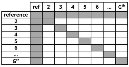
The possible input file combinations are summarized in Table 1:
The use of an input folder or directory (-d)
is recommended as it allows for new files to be added there in the future, reducing the computing required
for updated analyses. For instance, if a user does a first analysis with 5 input genomes today, it is possible
to check how the resulting clusters would change when adding an extra 10 genomes tomorrow, by copying these new 10
.faa / .gbk input files to the pre-existing -d folder, so that all previous BLAST searches are re-used.
In addition to .gbk and .faa files, the input directory can also contain one subfolder with pre-clustered sequences.
This feature was designed so that users can add previously produced get_homologues clusters,
or any other set of grouped sequences in FASTA format, to be analysed. For such a subfolder to be recognized, it must
be named subdir.clusters or subdir_. Sample data folder sample_buch_fasta/ contains such an example subfolder
which can be uncompressed to be tested. It is important to note that, during subsequent calculations,
these clusters are represented by the first sequence found in each. However, the output of the program will include
all pre-clustered sequences for convenience.
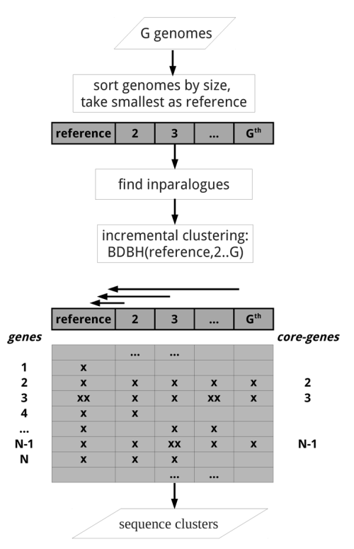
All remaining flags are options that can modify the default behavior of the program, which is to use the bidirectional best hit algorithm (BDBH) in order to compile clusters of potential orthologous ORFs, taking the smallest genome as a reference. By default protein sequences are used to guide the clustering, thus relying on BLASTP searches.
Perhaps the most important optional parameter would be the choice of clustering algorithm (Table 2):
|
|
The remaining options are now reviewed:
-v can be helpful after installation,
for it prints the enabled features of the program, which of course depend on the required and optional
binaries mentioned in sections 2.2 and 2.4.
-o is ideally used to submit to a computer cluster the required BLAST (and Pfam) searches, preparing a job for posterior
analysis on a single computer.
-c is used to request a pan- and core-genome analysis of the input genomes, which will be output as a tab-separated data file.
The number of samples for the genome composition analysis is set to 10 by default, but this can be edited at the header of
get_homologues.pl (check the $NOFSAMPLESREPORT variable). In addition, variables $MIN_PERSEQID_HOM and
$MIN_COVERAGE_HOM, with default values 0 and 20, respectively, control how homologues are called. Note that these are stringent values.
These can also be edited at lib/marfil_homology.pm to relax calling a sequence homologous, and therefore, redundant.
For instance, the equivalent values used by Tettelin and collaborators (PubMed=16172379),
are 50 and 50, respectively.
-R takes a number that will be used to seed the random generator used with option -c. By using the
same seed in different -c runs the user ensures that genomes are sampled in the same order.
-s can be used to reduce the memory footprint, provided that the Perl module
BerkeleyDB
is in place (please check section 2.4).
This option usually makes get_homologues slower, but for very large datasets or in machines with little memory resources
this might be the only way to complete a job.
-m allows the choice of runmode, which can be either -m local (the default),
-m cluster, for computing farms configured as explained in section 2.4) and
-m dryrun, which will allow you to run all required parallel jobs in batches manually.
Additionally -m /path/custom/HPC.conf can be used for cluster jobs that require a
custom HPC configuration file located elsewhere on the filesystem, useful for conda installs.
When combined with command-line tool ![[*]](crossref.png) parallel,
the dryrun mode can be used to parallelize the clustering tasks (isoforms, orthologues, inparalogues, see 4.2).
parallel,
the dryrun mode can be used to parallelize the clustering tasks (isoforms, orthologues, inparalogues, see 4.2).
-n sets the number of threads/CPUs to dedicate to each BLAST/HMMER job run locally, which by default is 2.
-I list_file.txt allows the user to restrict a get_homologues job to a subset of the genomes included in the input -d folder.
This flag can be used in conjunction with -c to control the order in which genomes are considered during pan- and core-genome analyses.
Taking the sample_buch_fasta folder, a valid list_file.txt could contain these lines:
Buch_aph_APS.faa
Buch_aph_Bp.faa
Buch_aph_Cc.faa
-X indicates that peptide similarity searches are to be performed with DIAMOND
(PubMed=25402007)
instead of BLASTP. This has a small sensitivity penalty
(see blog post),
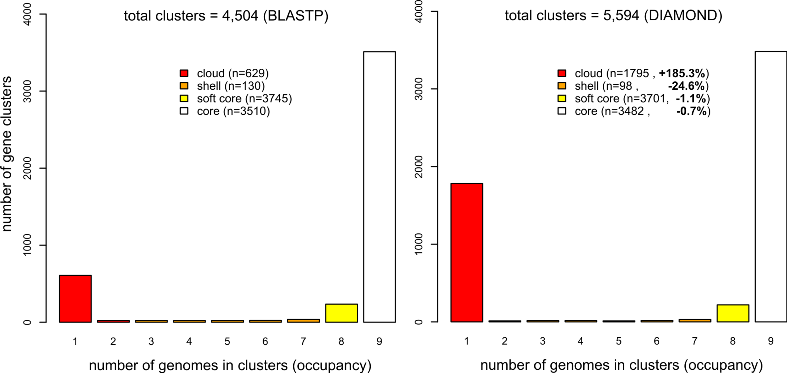
but the tests summarized in Table 3 show that it speeds up protein similarity searches
when compared to default BLAST jobs. The gain in computing time increases as more genomes are fed in,
allowing the analysis of even larger datasets (see Table 4).
Figure 4 shows that cloud clusters are where most of the differences arise when DIAMOND is used,
with more singletons produced than in BLASTP-based analysesi (see section 4.9.3 to learn how these plots can be produced).
|
|
|
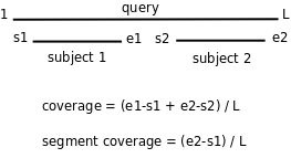
-C sets the minimum percentage of coverage required to call two sequences best hits,
as illustrated in the figure. The larger these values get, the smaller the chance that two sequences are
found to be reciprocal best hits. The default coverage value is set to 75%. When using the COGS algorithm
the maximum accepted coverage is 99%.
This parameter has a large impact on the results obtained and its optimal values will depend on the input
data and the anticipated use of the produced clusters.
-E sets the maximum expectation value (E-value) for BLAST alignments. This value is by default set to 1e-05.
This parameter might be adjusted for nucleotide BLAST searches or for very short proteins, under 40 residues.
-S can be passed to require a minimum % sequence identity for two sequences to be called best hits.
This option does not affect COGS runs; its default value is set to 1.
-N sets a minimum neighborhood correlation, as defined in
PubMed=18475320,
for two sequences to be called best hits. In this context 'neighborhood' is the set of homologous sequences reported by BLAST,
with the idea that two reliable best hits should have similar sets of homologous sequences.
-D is an extra restriction for calling best hits, that should have identical Pfam domain compositions. Note that this
option requires scanning all input sequences for Pfam domains, and this task requires some software to be installed (see section 2.4)
and extra computing time, ideally on a computer cluster (-m cluster).
While for BDBH domain filtering is done at the time bidirectional best hits are called, this processing step is performed only after the
standard OMCL and COGS algorithms have completed, to preserve each algorithm features.
|
-b reduces the number of pairwise BLAST searches performed while compiling core-genomes with algorithm BDBH,
reducing considerably memory and run-time requirements (for
|
-t is used to control which sequence clusters should be reported. By default only clusters which include at least one sequence
per genome are output. However, a value of -t 2 would report all clusters containing sequences from at least 2 taxa. A especial
case is -t 0, which will report all clusters found, even those with sequences from a single genome.
-a forces the program to extract user-selected sequence features typically contained in GenBank files, such as
tRNA or rRNA genes, instead of default CDSs. When using this option clusters are compiled by comparing nucleotide sequences
with BLASTN. Note that such BLASTN searches are expected to be less sensitive than default BLASTP searches.
-g can be used to request the compilation of clusters of intergenic sequences. This implies the calculation of ORF clusters and then
a search for pairs of 'orthologous' ORFs which flanking conserved intergenic regions, with the constraints set by three global variables in the
header of get_homologues.pl:
my $MININTERGENESIZE     = 200;   # minimum length (nts) required for intergenic
                                  # segments to be considered
my $MAXINTERGENESIZE     = 700;
my $INTERGENEFLANKORF    = 180;   # length in nts of intergene flanks borrowed
                                  # from neighbor ORFs

|
-f filters out cluster sequences with large differences in length. This flag
compares sequences within a cluster to the first (arbitrary) reference sequence. Those with length difference
(either shorter or longer) beyond the selected threshold will be removed. This might cause
the resulting cluster to be entirely removed if the final number of taxa falls below the -t minimum.
-r allows the choice of any input genome (of course included in -d folder)
as the reference, instead of the default smaller one. If possible, resulting clusters are named using gene names from
this genome, which can be used to select well annotated species for this purpose. In addition, when using the default
BDBH algorithm, the reference proteome is the one chosen to start adding genes in the clustering process. Therefore,
when using BDBH, the choice of reference proteome can have a large impact on the resulting number of clusters. By default,
the taxon with least genes is taken as reference. It is possible to change the way clusters are named by editing subroutine
extract_gene_name in file lib/phyTools.pm.
-e excludes clusters with inparalogues, defined as sequences with best hits in its own genome.
This option might be helpful to rule out clusters including several sequences from the same species, which might be of
interest for users employing these clusters for primer design, for instance.
-x allows COG-generated sequence clusters to contain the same sequence in more than one cluster.
-F is the inflation value that governs Markov Clustering in OMCL runs, as explained in
PubMed=12952885. As a rule of thumb,
low inflation values (-F 1)result in the inclusion of more sequences in fewer groups, whilst large values
produce more, smaller clusters (-F 4).
-A tells the program to produce a tab-separated file with average % sequence identity values among pairs of genomes,
computed from sequences in the final set of clusters (see also option -t ).
By default these identities are derived from BLASTP alignments, and hence correspond to amino acid sequence identities.
However, as explained earlier, option -a forces the program to use nucleotide sequences and run BLASTN
instead, and therefore, -a 'CDS' combined -A will produce genomic average nucleotide sequence identities (ANI), as used
in the literature to help define prokaryotic species
(PubMed=19855009).
-P tells the program to produce tab-separated files with
i) % of conserved protein clusters (POCP) and ii) Alignment Fraction (AF) shared by pairs of species.
POCP values are computed the following expression
(PubMed=24706738):

where  and
and  represent the conserved number of proteins in the two genomes being compared, respectively, and
  +and
+and  the total number of proteins in the two genomes being compared, respectively. These values are computed from sequences in the final set of clusters (see also option
 -t ).
By default these identities are derived from BLASTP alignments, and hence correspond to amino acid sequence identities. However, as explained earlier, option -a forces the program to use nucleotide sequences and run BLASTN instead, and therefore,
-a 'CDS' combined -A will produce percentage of conserved sequence (POCS) clusters.
AF values are computed following PubMed=26150420, using the same clustered sequences employed to compute POCP. While the original AF recipe divides the sum of the lengths of all BBH genes by the sum of the length of all the genes in each genome, in GET_HOMOLOGUES protein or CDS lengths are used instead.
-z can be called when performing a genome composition analysis with clustering algorithms OMCL or COGS.
In addition to the core- and pan-genome tab-separated files mentioned earlier (see option -c), this flag requests
a soft-core report, considering all sequence clusters present in a fraction of genomes defined by global variable $SOFTCOREFRACTION,
with a default value of 0.95. This choice produces a composition report more robust to assembly or annotation errors than the core-genome.
The following Perl scripts are included in the bundle to assist in the interpretation of results generated by get_homologues.pl:
In addition, two shell scripts are also included:
-A. From the latter type of matrix a distance matrix can optionally be calculated
to drive a neighbor joining tree. See example on section 4.9.1.
hclust() and heatmap.2() in order to produce a heatmap.
To check the options of any of these scripts please invoke them from the terminal with flag -h.
For instance, typing $ ./compare_clusters.pl -h in the terminal will produce the following:
-h 	 this message
-d 	 comma-separated names of cluster directories
-o 	 output directory
-n 	 use nucleotide sequence .fna clusters
-r 	 take first cluster dir as reference set, which might contain
   	 a single representative sequence per cluster
-s 	 use only clusters with syntenic genes
-t 	 use only clusters with single-copy orthologues from taxa >= t
-I 	 produce clusters with single-copy seqs from ALL taxa in file
-m 	 produce intersection pangenome matrices

-x 	 produce cluster report in OrthoXML format
-T 	 produce parsimony-based pangenomic tree
This section presents a few different ways of running get_homologues.pl and the accompanying scripts with provided sample input data.
This example takes the provided sample input folder sample_buch_fasta,
which contains the proteins sets of four
<1014>>http://en.wikipedia.org/wiki/Buchnera_and compiles clusters of BDBH sequences, which are candidates to be orthologues, with this command:
$ ./get_homologues.pl -d sample_buch_fasta .
The output should look like this (contained in file sample_output.txt):
# ./get_homologues.pl -i 0 -d sample_buch_fasta -o 0 -e 0 -f 0 -r 0 -t all -c 0 -I 0
# -m local -n 2 -M 0 -G 0 -P 0 -C 75 -S 1 -E 1e-05 -F 1.5 -N 0 -B 50 -s 0 -D 0 -g 0 -a '0' -x  -R 0

# results_directory=sample_buch_fasta_homologues
# parameters: MAXEVALUEBLASTSEARCH=0.01 MAXPFAMSEQS=250

# checking input files...
# Buch_aph_APS.faa 574
# Buch_aph_Bp.faa 507
# Buch_aph_Cc.faa 357
# Buch_aphid_Sg.faa 546

# 4 genomes, 1984 sequences

# taxa considered = 4 sequences = 1984 residues = 650959 MIN_BITSCORE_SIM = 17.2

# mask=BuchaphCc_f0_alltaxa_algBDBH_e0_ (_algBDBH)

# running makeblastdb with sample_buch_fasta_homologues/Buch_aph_APS.faa.fasta

# running makeblastdb with sample_buch_fasta_homologues/Buch_aph_Bp.faa.fasta

# running makeblastdb with sample_buch_fasta_homologues/Buch_aph_Cc.faa.fasta

# running makeblastdb with sample_buch_fasta_homologues/Buch_aphid_Sg.faa.fasta

# running BLAST searches ...
# done

# concatenating and sorting blast results...
# sorting _Buch_aph_APS.faa results (0.12MB)
# sorting _Buch_aph_Bp.faa results (0.11MB)
# sorting _Buch_aph_Cc.faa results (0.084MB)
# sorting _Buch_aphid_Sg.faa results (0.11MB)
# done


# parsing blast result! (sample_buch_fasta_homologues/tmp/all.blast , 0.42MB)
# parsing blast file finished

# creating indexes, this might take some time (lines=9.30e+03) ...

# construct_taxa_indexes: number of taxa found = 4
# number of file addresses = 9.3e+03 number of BLAST queries  = 2.0e+03

# clustering orthologous sequences

# clustering inparalogues in Buch_aph_Cc.faa (reference)
# 0 sequences

# clustering inparalogues in Buch_aph_APS.faa
# 1 sequences

# finding BDBHs between Buch_aph_Cc.faa and Buch_aph_APS.faa
# 324 sequences

# clustering inparalogues in Buch_aph_Bp.faa
# 0 sequences

# finding BDBHs between Buch_aph_Cc.faa and Buch_aph_Bp.faa
# 326 sequences

# clustering inparalogues in Buch_aphid_Sg.faa
# 0 sequences

# finding BDBHs between Buch_aph_Cc.faa and Buch_aphid_Sg.faa
# 317 sequences

# looking for valid ORF clusters (n_of_taxa=4)...


# number_of_clusters = 305
# cluster_list = sample_buch_fasta_homologues/BuchaphCc_f0_alltaxa_algBDBH_e0_.cluster_list
# cluster_directory = sample_buch_fasta_homologues/BuchaphCc_f0_alltaxa_algBDBH_e0_

# runtime: 64 wallclock secs ( 0.74 usr  0.08 sys + 61.49 cusr  0.47 csys = 62.78 CPU)
# RAM use: 20.3 MB
In summary, the output details the processing steps required:
Buch_aph_APS.faa,Buch_aph_Bp.faa,Buch_aph_Cc.faa,Buch_aphid_Sg.faa),
which contain 574, 507, 357 and 546 protein sequences, respectively. In total there are
four input taxa and 1984 sequences.
sample_buch_fasta_homologues/BuchaphCc_f0_alltaxa_algBDBH_e0_ together with
file sample_buch_fasta_homologues/BuchaphCc_f0_alltaxa_algBDBH_e0_.cluster_list, which lists the found
clusters and their taxa composition. It can be seen that the folder name contains the key settings used to
cluster the sequences contained therein:
BuchaphCc_f0_alltaxa_algBDBH_e0_
|         |  |       |       |
|         |  |       |       -e option was not used (inparalogues are in)
|         |  |       the clustering algorithm is BDBD (default)
|         |  all clusters contain at least 1 sequence from each taxa (default -t behavior)
|         -f option not used (no length filtering)
reference proteome
In this case a total of 305 protein sequence clusters are produced, which include the original FASTA headers plus information of which segment was actually aligned by BLAST for inclusion in the cluster:
>gi|116515296| Rho [Buchnera aphidicola str. Cc (Cinara cedri)] | aligned:1-419 (420)
MNLTKLKNTSVSKLIILGEKIGLENLARMRKQDIIFSILKQHSKSGEDIFGDGVLEILQDGFGFLRSSDSSYLAGPDDIYVSPS...
>gi|15617182| termination factor Rho [Buchnera aphidicola str. APS] | aligned:1-419 (419)
MNLTALKNMPVSELITLGEKMGLENLARMRKQDIIFAILKQHAKSGEDIFGDGVLEILQDGFGFLRSADSSYLAGPDDIYVSPS...
>gi|27905006| termination factor Rho [Buchnera aphidicola str. Bp] | aligned:1-419 (419)
MNLTALKNIPVSELIFLGDNAGLENLARMRKQDIIFSILKQHAKSGEDIFGDGVLEILQDGFGFLRSSDSSYLAGPDDIYVSPS...
>gi|21672828| termination factor Rho [Buchnera aphidicola str. Sg] | aligned:1-419 (419)
MNLTALKNMPVSELITLGEKMGLENLARMRKQDIIFAILKQHAKSGEDIFGDGVLEILQDGFGFLRSADSSYLAGPDDIYVSPS...
If we wanted to test a different sequence clustering algorithm we could run
$ ./get_homologues.pl -d sample_buch_fasta -G ,
which will produce 298 clusters
employing the COG triangles algorithm (see Table 2) in folder
sample_buch_fasta_homologues/BuchaphCc_f0_alltaxa_algCOG_e0_.
Furthermore, typing $ ./get_homologues.pl -d sample_buch_fasta -M
produces 308 clusters employing the OMCL algorithm in folder
sample_buch_fasta_homologues/BuchaphCc_f0_alltaxa_algOMCL_e0_.
Now we can make use of script compare_clusters.pl to get the intersection between these cluster sets and choose only the consensus subset. We will need to type (without any blanks between folder names, in a single long line) and execute:
./compare_clusters.pl -o sample_intersection -d \
sample_buch_fasta_homologues/BuchaphCc_f0_alltaxa_algBDBH_e0_, \
sample_buch_fasta_homologues/BuchaphCc_f0_alltaxa_algCOG_e0_, \
sample_buch_fasta_homologues/BuchaphCc_f0_alltaxa_algOMCL_e0_
The following output is produced:
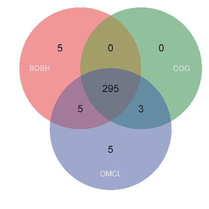
# number of input cluster directories = 3

# parsing clusters in sample_buch_fasta_homologues/BuchaphCc_f0_alltaxa_algBDBH_e0_ ...
# cluster_list in place, will parse it (BuchaphCc_f0_alltaxa_algBDBH_e0_.cluster_list)
# number of clusters = 305
# parsing clusters in sample_buch_fasta_homologues/BuchaphCc_f0_alltaxa_algCOG_e0_ ...
# cluster_list in place, will parse it (BuchaphCc_f0_alltaxa_algCOG_e0_.cluster_list)
# number of clusters = 298
# parsing clusters in sample_buch_fasta_homologues/BuchaphCc_f0_alltaxa_algOMCL_e0_ ...
# cluster_list in place, will parse it (BuchaphCc_f0_alltaxa_algOMCL_e0_.cluster_list)
# number of clusters = 308

# intersection output directory: sample_intersection

# intersection size = 295 clusters

# intersection list = sample_intersection/intersection_t0.cluster_list

# input set: sample_intersection/BuchaphCc_f0_alltaxa_algBDBH_e0_.venn_t0.txt
# input set: sample_intersection/BuchaphCc_f0_alltaxa_algCOG_e0_.venn_t0.txt
# input set: sample_intersection/BuchaphCc_f0_alltaxa_algOMCL_e0_.venn_t0.txt

# Venn diagram = sample_intersection/venn_t0.pdf
# Venn region file: sample_intersection/unique_BuchaphCc_f0_alltaxa_algBDBH_e0_.venn_t0.txt (5)
# Venn region file: sample_intersection/unique_BuchaphCc_f0_alltaxa_algCOG_e0_.venn_t0.txt (0)
# Venn region file: sample_intersection/unique_BuchaphCc_f0_alltaxa_algOMCL_e0_.venn_t0.txt (5)
The 295 resulting clusters, those present in all input cluster sets, are placed in a new folder
which was designated by parameter -o sample_intersection. Note that these are clusters that belong to
the core-genome, as they contain sequence from all input taxa. A Venn diagram,
such as the one in Figure 8, might also be produced which summarizes the analysis.
|
If we are interested only in clusters containing single-copy proteins from all input species,
as they are probably safer orthologues, we can add the option -t 4 to our previous command,
as our example dataset contains 4 input proteomes.
This example takes the sample input folder sample_buch_fasta,
and demonstrates how you could run a large analysis on a multicore Linux box, not a computer cluster.
This example requires command-line tool parallel,
which in Ubuntu can be installed with sudo apt-get -y install:
# 1) run BLASTN (and HMMER) in batches
./get_homologues-est.pl -d sample_buch_fasta -o

# 2) run in -m dryrun mode
./get_homologues-est.pl -d sample_buch_fasta -m dryrun
# ...
# EXIT: check the list of pending commands at sample_buch_fasta_homologues/dryrun.txt
parallel < sample_buch_fasta_homologues/dryrun.txt

# repeat 2) until completion
./get_homologues-est.pl -d sample_buch_fasta -m dryrun
# ...
A similar analysis could be performed with a single input FASTA file containing amino acid sequences, provided that each contains a [taxon name] in its header, as explained in section 3.1:
>gi|10957100|ref|NP_057962.1| ... [Buchnera aphidicola str. APS (Acyrthosiphon pisum)]
MFLIEKRRKLIQKKANYHSDPTTVFNHLCGSRPATLLLETAEVNKKNNLESIMIVDSAIRVSAVKNSVKI
TALSENGAEILSILKENPHKKIKFFEKNKSINLIFPSLDNNLDEDKKIFSLSVFDSFRFIMKSVNNTKRT
SKAMFFGGLFSYDLISNFESLPNVKKKQKCPDFCFYLAETLLVVDHQKKTCLIQSSLFGRNVDEKNRIKK
RTEEIEKKLEEKLTSIPKNKTTVPVQLTSNISDFQYSSTIKKLQKLIQKGEIFQVVPSRKFFLPCDNSLS
AYQELKKSNPSPYMFFMQDEDFILFGASPESSLKYDEKNRQIELYPIAGTRPRGRKKDGTLDLDLDSRIE
LEMRTNHKELAEHLMLVDLARNDLARICEPGSRYVSDLVKVDKYSHVMHLVSKVVGQLKYGLDALHAYSS
CMNMGTLTGAPKVRAMQLIAEYEGEGRGSYGGAIGYFTDLGNLDTCITIRSAYVESGVATIQAGAGVVFN
SIPEDEVKESLNKAQAVINAIKKAHFTMGSS
[...]
>gi|15616637|ref|NP_239849.1| ... [Buchnera aphidicola str. APS (Acyrthosiphon pisum)]
MTSTKEIKNKIVSVTNTKKITKAMEMVAVSKMRKTEERMRSGRPYSDIIRKVIDHVTQGNLEYKHSYLEE
RKTNRIGMIIISTDRGLCGGLNTNLFKQVLFKIQNFAKVNIPCDLILFGLKSLSVFKLCGSNILAKATNL
GENPKLEELINSVGIILQEYQCKRIDKIFIAYNKFHNKMSQYPTITQLLPFSKKNDQDASNNNWDYLYEP
ESKLILDTLFNRYIESQVYQSILENIASEHAARMIAMKTATDNSGNRIKELQLVYNKVRQANITQELNEI
VSGASAVSID
[...]
>gi|21672839|ref|NP_660906.1| ... [Buchnera aphidicola str. Sg (Schizaphis graminum)]
MHLNKMKKVSLKTYLVLFFLIFFIFCSFWFIKPKEKKLKLEKLRYEEVIKKINAKNNQNLKSVENFITEN
KNIYGTLSSLFLAKKYILDKNLDKALIQLNNSLKYTKEENLQNILKIRIAKIKIQQNKNQDAIKILEEIK
DNSWKNIVENMKGDIFMKNKEIKKAILAWKKSKYLEKSNASKEIINMKINEIKR
It is possible to analyze the provided sample input file sample_buchnera.faa with the following command:
$ ./get_homologues.pl -i sample_buchnera.faa .
Obtaining:
# results_directory=sample_buchnera_homologues
# parameters: MAXEVALUEBLASTSEARCH=0.01 MAXPFAMSEQS=250

# checking input files...
# sample_buchnera.faa

# created file sample_buchnera_homologues/tmp/all.fa (4 genomes, 1984 sequences)

# taxa considered = 4 sequences = 1984 residues = 650959 MIN_BITSCORE_SIM = 17.2

# mask=BuchneraaphidicolastrCcCinaracedri3_f0_alltaxa_algBDBH_e0_ (_algBDBH)

# running makeblastdb with sample_buchnera_homologues/tmp/all.fa
# running local BLAST search
# done


# parsing blast result! (sample_buchnera_homologues/tmp/all.blast , 0.44MB)
# parsing blast file finished

# creating indexes, this might take some time (lines=9.30e+03) ...

# construct_taxa_indexes: number of taxa found = 4
# number of file addresses = 9.3e+03 number of BLAST queries  = 2.0e+03

# clustering orthologous sequences

# clustering inparalogues in Buchnera_aphidicola_str__Cc__Cinara_cedri__3.faa (reference)
# 0 sequences

[...]

# looking for valid ORF clusters (n_of_taxa=4)...


# number_of_clusters = 305
# cluster_list = [...]/BuchneraaphidicolastrCcCinaracedri3_f0_alltaxa_algBDBH_e0_.cluster_list
# cluster_directory = [...]/BuchneraaphidicolastrCcCinaracedri3_f0_alltaxa_algBDBH_e0_

# runtime: 55 wallclock secs ( 0.76 usr  0.04 sys + 51.75 cusr  0.23 csys = 52.78 CPU)
# RAM use: 21.3 MB
The use of input files in GenBank format allows clustering nucleotide sequences in addition
to proteins, since this format supports the annotation of raw genomic sequences.
This example illustrates this feature by taking the input folder
sample_plasmids_gbk, which contains 12 GenBank files of plasmid replicons,
which we analyze by running $ ./get_homologues.pl -d sample_plasmids_gbk :
# results_directory=sample_plasmids_gbk_homologues
# parameters: MAXEVALUEBLASTSEARCH=0.01 MAXPFAMSEQS=250

# checking input files...
# E_coli_ST131_plasmid_pKC394.gb 55
# E_coli_plasmid_pMUR050.gb 60
# IncN_plasmid_R46.gb 63
# K_oxytoca_plasmid_pKOX105.gb 69
# K_pneumoniae_12_plasmid_12.gb 92
# K_pneumoniae_9_plasmid_9.gb 87
# K_pneumoniae_KP96_plasmid_pKP96.gb 64
# S_enterica_subsp_enterica_serovar_Dublin_plasmid_pMAK2.gb 52
# Uncultured_bacterium_plasmid_pRSB201.gb 58
# Uncultured_bacterium_plasmid_pRSB203.gb 49
# Uncultured_bacterium_plasmid_pRSB205.gb 52
# Uncultured_bacterium_plasmid_pRSB206.gb 55

# 12 genomes, 756 sequences

# taxa considered = 12 sequences = 756 residues = 184339 MIN_BITSCORE_SIM = 16.0

# mask=EcoliplasmidpMUR050_f0_alltaxa_algBDBH_e0_ (_algBDBH)

[..]
# running BLAST searches ...
# done

# concatenating and sorting blast results...
# sorting _E_coli_ST131_plasmid_pKC394.gb results (0.026MB)
# sorting _E_coli_plasmid_pMUR050.gb results (0.026MB)
# sorting _IncN_plasmid_R46.gb results (0.026MB)
# sorting _K_oxytoca_plasmid_pKOX105.gb results (0.031MB)
# sorting _K_pneumoniae_12_plasmid_12.gb results (0.036MB)
# sorting _K_pneumoniae_9_plasmid_9.gb results (0.027MB)
# sorting _K_pneumoniae_KP96_plasmid_pKP96.gb results (0.026MB)
# sorting _S_enterica_subsp_enterica_serovar_Dublin_plasmid_pMAK2.gb results (0.025MB)
# sorting _Uncultured_bacterium_plasmid_pRSB201.gb results (0.029MB)
# sorting _Uncultured_bacterium_plasmid_pRSB203.gb results (0.023MB)
# sorting _Uncultured_bacterium_plasmid_pRSB205.gb results (0.026MB)
# sorting _Uncultured_bacterium_plasmid_pRSB206.gb results (0.026MB)
# done


# parsing blast result! (sample_plasmids_gbk_homologues/tmp/all.blast , 0.33MB)
# parsing blast file finished

# creating indexes, this might take some time (lines=7.61e+03) ...

# construct_taxa_indexes: number of taxa found = 12
# number of file addresses = 7.6e+03 number of BLAST queries  = 7.6e+02

# clustering orthologous sequences

# clustering inparalogues in E_coli_plasmid_pMUR050.gb (reference)
# 2 sequences

[...]
# looking for valid ORF clusters (n_of_taxa=12)...


# number_of_clusters = 24
# cluster_list = [...]_homologues/EcoliplasmidpMUR050_f0_alltaxa_algBDBH_e0_.cluster_list
# cluster_directory = sample_plasmids_gbk_homologues/EcoliplasmidpMUR050_f0_alltaxa_algBDBH_e0_
This outcome is similar to that explained in example 4.1, with the notable difference
that now both protein and nucleotide sequence clusters (24) are produced, as GenBank files usually contain both types
of sequences. File EcoliplasmidpMUR050_f0_alltaxa_algBDBH_e0_.cluster_list.cluster_list
summarizes the contents and composition of the clusters stored in folder
EcoliplasmidpMUR050_f0_alltaxa_algBDBH_e0_.
For instance, the data concerning cluster 100_traJ looks like this:
cluster 100_traJ size=12 taxa=12 file: 100_traJ.faa dnafile: 100_traJ.fna
: E_coli_plasmid_pMUR050.gb
: E_coli_ST131_plasmid_pKC394.gb
: IncN_plasmid_R46.gb
: K_oxytoca_plasmid_pKOX105.gb
: K_pneumoniae_12_plasmid_12.gb
: K_pneumoniae_9_plasmid_9.gb
: K_pneumoniae_KP96_plasmid_pKP96.gb
: S_enterica_subsp_enterica_serovar_Dublin_plasmid_pMAK2.gb
: Uncultured_bacterium_plasmid_pRSB201.gb
: Uncultured_bacterium_plasmid_pRSB203.gb
: Uncultured_bacterium_plasmid_pRSB205.gb
: Uncultured_bacterium_plasmid_pRSB206.gb
The two FASTA files produced for this cluster are now dissected.
Note that each header includes the coordinates of the sequence in the context of a genomic contig.
For instance, the first sequence was extracted from the leading strand of GenBank contig AY522431,
positions 44726-46255, out of a total 56634 nucleotides. Furthermore, the names of neighboring genes
are annotated when available, in order to capture some synteny information. These syntenic data
can be valuable when evaluating possible orthologous genes, as conservation of genomic position (also
operon context) strongly suggests orthology among prokaryots:
ID:ABG33824.1 |[Escherichia coli]||traJ|1530|AY522431(56634):44726-46255:-1 [...]|neighbour_genes:traI,traK|
ATGGACGATAGAGAAAGAGGCTTAGCATTTTTATTTGCAATTACTTTGCCTCCAGTGATGGTATGGTTTCTAGTT...
[...]
and
>ID:ABG33824.1 |[Escherichia coli]||traJ|1530|AY522431(56634):44726-46255:-1 [...] | aligned:1-509 (509)
MDDRERGLAFLFAITLPPVMVWFLV...
The BDBH algorithm in get_homologues.pl can be modified by requiring bidirectional best hits to
share the same domain architecture, annotated in terms of Pfam domains. For large volumes of sequences
this task should be accomplished on a computer cluster, but of course can also be performed locally.
The command on the terminal could then be: $ ./get_homologues.pl -d sample_plasmids_gbk -D
The generated output should be:
# results_directory=sample_plasmids_gbk_homologues
# parameters: MAXEVALUEBLASTSEARCH=0.01 MAXPFAMSEQS=250

# checking input files...
# E_coli_ST131_plasmid_pKC394.gb 55
# E_coli_plasmid_pMUR050.gb 60
# IncN_plasmid_R46.gb 63
# K_oxytoca_plasmid_pKOX105.gb 69
# K_pneumoniae_12_plasmid_12.gb 92
# K_pneumoniae_9_plasmid_9.gb 87
# K_pneumoniae_KP96_plasmid_pKP96.gb 64
# S_enterica_subsp_enterica_serovar_Dublin_plasmid_pMAK2.gb 52
# Uncultured_bacterium_plasmid_pRSB201.gb 58
# Uncultured_bacterium_plasmid_pRSB203.gb 49
# Uncultured_bacterium_plasmid_pRSB205.gb 52
# Uncultured_bacterium_plasmid_pRSB206.gb 55

# 12 genomes, 756 sequences

# taxa considered = 12 sequences = 756 residues = 184339 MIN_BITSCORE_SIM = 16.0

# mask=EcoliplasmidpMUR050_f0_alltaxa_algBDBH_Pfam_e0_ (_algBDBH_Pfam)

# skipped genome parsing (sample_plasmids_gbk_homologues/tmp/selected.genomes)


# submitting Pfam HMMER jobs ...
[...]
# done

# concatenating Pfam files ([...]/_E_coli_ST131_plasmid_pKC394.gb.fasta.pfam)...
# done

[..]

# parsing Pfam domain assignments (generating sample_plasmids_gbk_homologues/tmp/all.pfam) ...

# skip BLAST searches and parsing

# WARNING: please remove/rename results directory:
# '/home/contrera/codigo/cvs/get_homologues/sample_plasmids_gbk_homologues/'
# if you change the sequences in your .gbk/.faa files or want to re-run

# creating indexes, this might take some time (lines=7.61e+03) ...

# construct_taxa_indexes: number of taxa found = 12
# number of file addresses = 7.6e+03 number of BLAST queries  = 7.6e+02

# creating Pfam indexes, this might take some time (lines=7.54e+02) ...


# clustering orthologous sequences

# clustering inparalogues in E_coli_plasmid_pMUR050.gb (reference)
# 2 sequences (re-using previous results)

[...]

# looking for valid ORF clusters (n_of_taxa=12)...


# number_of_clusters = 24
# cluster_list = [...]/EcoliplasmidpMUR050_f0_alltaxa_algBDBH_Pfam_e0_.cluster_list
# cluster_directory = sample_plasmids_gbk_homologues/EcoliplasmidpMUR050_f0_alltaxa_algBDBH_Pfam_e0_
Matching Pfam domains are summarized in the .cluster_list file, with this format:
cluster 606_.. size=8 taxa=8 Pfam=PF04471, file: 606_...faa 606_...fna
The sequence clusters derived from a set of GenBank files can be further processed in order to select those that contain only syntenic genes, defined as those having at least one neighbor included in other clusters. Again we will invoke script compare_clusters.pl for this task:
./compare_clusters.pl -o sample_intersection -s -d \
sample_plasmids_gbk_homologues/EcoliplasmidpMUR050_f0_alltaxa_algBDBH_e0_
The following output is produced:
# number of input cluster directories = 1

# parsing clusters in sample_plasmids_gbk_homologues/EcoliplasmidpMUR050_f0_alltaxa_algBDBH_e0_ ...
# cluster_list in place, will parse it ([...]/EcoliplasmidpMUR050_f0_alltaxa_algBDBH_e0_.cluster_list)
# number of clusters = 24

# intersection output directory: sample_intersection

# intersection size = 21 clusters (syntenic)

# intersection list = sample_intersection/intersection_t0_s.cluster_list
|
Sometimes we will need to compare clusters of possibly orthologous sequences, produced by get_homologues.pl
in any of the ways explained earlier, with a set of sequences defined elsewere, for instance in a publication.
This can be done to validate a set of core clusters and to check that nothing important was left out.
We can accomplish just this with help from script compare_clusters.pl, invoking option -r,
which indicates that the first parsed cluster folder is actually a reference to be compared.
To illustrate this application we have set a folder with 4 protein sequences from Buchnera aphidicola from strain Cinara cedri
(directory sample_buch_fasta/sample_proteins), each sequence in a single FASTA file. Note that these clusters must contain
sequences contained in the larger dataset which we want to compare with, otherwise the script will not match them. Headers are not
used by the program, only the sequences matter.
In order to check whether these sequences are clustered in any of the clusters generated earlier, say with BDBH, we will issue a command such as:
./compare_clusters.pl -o sample_intersection -r -d \
sample_buch_fasta/sample_proteins,\
sample_buch_fasta_homologues/BuchaphCc_f0_alltaxa_algBDBH_e0_\
The following output should be produced:
# number of input cluster directories = 2

# parsing clusters in sample_buch_fasta/sample_proteins ...
# no cluster list in place, checking directory content ...
# WARNING: [taxon names] will be automatically extracted from FASTA headers,
# please watch out for errors

# number of clusters = 4
# parsing clusters in sample_buch_fasta_homologues/BuchaphCc_f0_alltaxa_algBDBH_e0_ ...
# cluster_list in place, will parse it ([...]/BuchaphCc_f0_alltaxa_algBDBH_e0_.cluster_list)
# number of clusters = 305

# intersection output directory: sample_intersection

# intersection size = 4 clusters

# intersection list = sample_intersection/intersection_t0.cluster_list

# input set: sample_intersection/sample_proteins.venn_t0.txt
# input set: sample_intersection/BuchaphCc_f0_alltaxa_algBDBH_e0_.venn_t0.txt

# Venn diagram = sample_intersection/venn_t0.pdf
# Venn region file: sample_intersection/unique_sample_proteins.venn_t0.txt (0)
# Venn region file: sample_intersection/unique_BuchaphCc_f0_alltaxa_algBDBH_e0_.venn_t0.txt (301)
The use of input files in GenBank format also allows the extraction of clusters
of flanked orthologous intergenic regions, which might be of interest as these are expected to
mutate at higher rates compared to coding sequences. In this example this feature is
illustrated by processing folder sample_plasmids_gbk with options
-g -I sample_plasmids_gbk/include_list.txt
The restraints that apply to the parsed
intergenic regions are defined by three global variables variables within get_homologues.pl,
as explained in section 3.4. These default values might be edited for specific tasks;
for instance, chloroplast intergenic regions are usually much smaller than 200 bases, the default size,
and therefore variable $MININTERGENESIZE should be set to a smaller value.
Moreover, in this example we restrict the search for conserved intergenic segments to
Klebsiella pneumoniae plasmids,
by creating a file sample_plasmids_gbk/include_list.txt with these contents:
K_pneumoniae_12_plasmid_12.gb
K_pneumoniae_9_plasmid_9.gb
K_pneumoniae_KP96_plasmid_pKP96.gb
We can now execute
$ ./get_homologues.pl -d sample_plasmids_gbk -g -I sample_plasmids_gbk/include_list.txt:
# results_directory=sample_plasmids_gbk_homologues
# parameters: MAXEVALUEBLASTSEARCH=0.01 MAXPFAMSEQS=250

# checking input files...
# E_coli_ST131_plasmid_pKC394.gb 55 (intergenes=7)
# E_coli_plasmid_pMUR050.gb 60 (intergenes=12)
# IncN_plasmid_R46.gb 63 (intergenes=11)
# K_oxytoca_plasmid_pKOX105.gb 69 (intergenes=13)
# K_pneumoniae_12_plasmid_12.gb 92 (intergenes=11)
# K_pneumoniae_9_plasmid_9.gb 87 (intergenes=12)
# K_pneumoniae_KP96_plasmid_pKP96.gb 64 (intergenes=18)
# S_enterica_subsp_enterica_serovar_Dublin_plasmid_pMAK2.gb 52 (intergenes=9)
# Uncultured_bacterium_plasmid_pRSB201.gb 58 (intergenes=9)
# Uncultured_bacterium_plasmid_pRSB203.gb 49 (intergenes=7)
# Uncultured_bacterium_plasmid_pRSB205.gb 52 (intergenes=8)
# Uncultured_bacterium_plasmid_pRSB206.gb 55 (intergenes=10)

# 12 genomes, 756 sequences

# included input files (3):
: K_pneumoniae_12_plasmid_12.gb K_pneumoniae_12_plasmid_12.gb 92
: K_pneumoniae_9_plasmid_9.gb K_pneumoniae_9_plasmid_9.gb 87
: K_pneumoniae_KP96_plasmid_pKP96.gb K_pneumoniae_KP96_plasmid_pKP96.gb 64

[...]

# looking for valid ORF clusters (n_of_taxa=3)...


# number_of_clusters = 32
# cluster_list = sample_plasmids_gbk_homologues/[...]include_list.txt_algBDBH_e0_.cluster_list
# cluster_directory = sample_plasmids_gbk_homologues/[...]include_list.txt_algBDBH_e0_

# looking for valid clusters of intergenic regions (n_of_taxa=3)...
# parameters: MININTERGENESIZE=200 MAXINTERGENESIZE=700 INTERGENEFLANKORF=180


# number_of_intergenic_clusters = 1
# intergenic_cluster_list = [...]/[...]_intergenic200_700_180_.cluster_list
# intergenic_cluster_directory = sample_plasmids_gbk_homologues/[...]_intergenic200_700_180_

# runtime:  1 wallclock secs ( 0.10 usr  0.01 sys +  0.05 cusr  0.01 csys =  0.17 CPU)
# RAM use: 27.6 MB
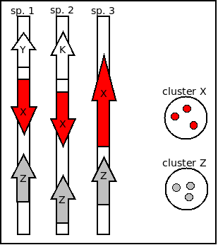
Intergenic clusters, illustrated by Figure 3.4, include upper-case nucleotides to mark up the sequence of flanking ORFs, with the intergenic region itself in lower-case, and the names of the flanking ORFs in the FASTA header, with their strand in parentheses:
>1 | intergenic18|coords:63706..64479|length:774|neighbours:ID:ABY74399.1(-1),ID:ABY74398.1(1)...
CGCGCCATTGCTGGCCTGAAGGTATTCCCAATACCCTCCCTGGTAGTCTTTAGCGTAACGATTCAGAAAGGACTGAATGAAGTGATCTGCGCTGAAGAAAGCG
CCACGAAATGCCGCAGGCATGAAGTTCATGCGGGCGTTTTCAGAAATGTAGCGGGCGGTGATTTCGATAGTTTCCATgatacttcctctttaagccgataccg
gcgatggttaagcggcaggcacatcacctgccactttttaattatcgtacaatggggcgttaaagtcaatacaagtacggattatatttacctaattttatgc
ccgtcagagcatggaaggcgacctcgccggactccaccggacaccgggggcaaatcgccggaaactgcgggactgaccggagcgacaggccacccccctccct
gctagcccgccgccacgcggccggttacaggggacactgagaaagcagaaagccaacaaacactatatatagcgttcgttggcagctgaagcagcactacata
tagtagagtacctgtaaaacttgccaacctgaccataacagcgatactgtataagtaaacagtgatttggaagatcgctATGAAGGTCGATATTTTTGAAAGC
TCCGGCGCCAGCCGGGTACACAGCATCCCTTTTTATCTGCAAAGAATTTCTGCGGGGTTCCCCAGCCCGGCCCAGGGCTATGAAAAGCAGGAGTTAAACCTGC
ATGAGTATTGTGTTCGTCACCCTTCAGCAACTTACTTCCTGCGGGTTTCTGGC
>2 | intergenic3|coords:9538..10293|length:756|neighbours:ID:ACI62996.1(-1),ID:ACI62997.1(1)...
CGCGCCATTGCTGGCCTGAAGGTATTCCCAATACCCTCCCTGGTAGTCTTTAGCGTAACGATTCAGAAAGGACTGAATGAAGTGATCTGCGCTGAAGAAAGCG
CCACGAAATGCCGCAGGCATGAAGTTCATGCGGGCGTTTTCAGAAATGTAGCGGGCGGTGATTTCGATAGTTTCCATgatacttcctctttaagccgataccg
gcgatggttaagcggcaggcacatcacctgccactttttaattatcgtacaatggggcgttaaagtcaatacaagtacggattatatttacctaattttatgc
ccgtcagagcatggaaggcgacctcgccggactccaccggacaccgggggcaaatcgccggaaactgcgggactgaccggagcgacaggccacccccctccct
gctagcccgccgccacgcggccggttacaggggacactgagaaagcagaaagccaacaaacactatatatagcgttcgttggcagctgaagcagcactacata
tagtagagtacctgtaaaacttgccaacctgaccataacagcgatactgtataagtaaacaGTGATTTGGAAGATCGCTATGAAGGTCGATATTTTTGAAAGC
TCCGGCGCCAGCCGGGTACACAGCATCCCTTTTTATCTGCAAAGAATTTCTGCGGGGTTCCCCAGCCCGGCCCAGGGCTATGAAAAGCAGGAGTTAAACCTGC
ATGAGTATTGTGTTCGTCACCCTTCAGCAACTTAC
...
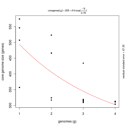
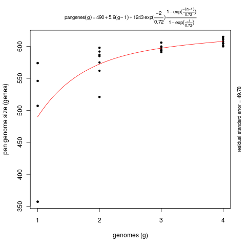
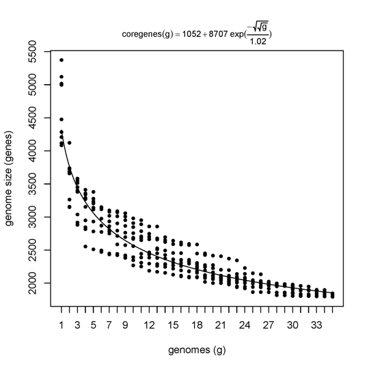
The next few examples illustrate how get_homologues.pl might be used to analyze the genomic evolution of a group of related organisms, the core-genome and the pan-genome, using the terms coined by Tettelin and collaborators (PubMed=16172379).
First we will try option -t 0 in combination with the OMCL or the COG algorithms.
By enforcing this option we are actually asking for all possible clusters, including those which might not
contain sequences from all input genomes (taxa). For this reason the use of this option usually means
that a large number of clusters are reported. This is particularly true for COG runs, since this algorithm
does not resolve clusters involving less than 3 genomes. The default algorithm BDBH is not available with this option.
For instance, by calling
$ ./get_homologues.pl -d sample_plasmids_gbk -t 0 -G we obtain 199 clusters:
[...]
# looking for valid ORF clusters (n_of_taxa=0)...

# number_of_clusters = 199
# cluster_list = [...]/UnculturedbacteriumplasmidpRSB203_f0_0taxa_algCOG_e0_.cluster_list
# cluster_directory = [...]/UnculturedbacteriumplasmidpRSB203_f0_0taxa_algCOG_e0_
By choosing the OMCL algorithm we obtain a smaller set of clusters, which we can test by typing on the terminal
$ ./get_homologues.pl -d sample_plasmids_gbk -t 0 -M:
[...]
# looking for valid ORF clusters (n_of_taxa=0)...

# number_of_clusters = 193
# cluster_list = [...]/UnculturedbacteriumplasmidpRSB203_f0_0taxa_algOMCL_e0_.cluster_list
# cluster_directory = [...]/UnculturedbacteriumplasmidpRSB203_f0_0taxa_algOMCL_e0_
We can now take advantage of script compare_clusters.pl, and the generated cluster directories, to compile the corresponding pangenome matrix. This can be accomplished for a single cluster set:
./compare_clusters.pl -o sample_intersection -m -d \
sample_plasmids_gbk_homologues/Uncultured[...]_f0_0taxa_algCOG_e0_
or for the intersection of several sets, in order to get a consensus pangenome matrix:
./compare_clusters.pl -o sample_intersection -m -d \
sample_plasmids_gbk_homologues/Uncultured[...]_f0_0taxa_algCOG_e0_,\
sample_plasmids_gbk_homologues/Uncultured[...]_f0_0taxa_algOMCL_e0_
The ouput of the latter command will include the following lines:
[...]

# number of input cluster directories = 2

# parsing clusters in sample_plasmids_gbk_homologues/Uncultured[...]_f0_0taxa_algCOG_e0_ ...
# cluster_list in place, will parse it ([...]/Uncultured[...]_f0_0taxa_algCOG_e0_.cluster_list)
# WARNING: cluster 62_transposase.faa duplicate59_transposase.faa
# WARNING: cluster 116_tnpA.faa duplicates 59_transposase.faa
# number of clusters = 196 duplicated = 3
# parsing clusters in sample_plasmids_gbk_homologues/Uncultured[...]_f0_0taxa_algOMCL_e0_ ...
# cluster_list in place, will parse it ([...]/Uncultured[...]_f0_0taxa_algOMCL_e0_.cluster_list)
# number of clusters = 193 duplicated = 0

[...]

# intersection size = 180 clusters

# intersection list = sample_intersection/intersection_t0.cluster_list

# pangenome_file = sample_intersection/pangenome_matrix_t0.tab \
   transposed = sample_intersection/pangenome_matrix_t0.tr.tab
# pangenome_genes = sample_intersection/pangenome_matrix_genes_t0.tab \
   transposed = sample_intersection/pangenome_matrix_genes_t0.tr.tab
# pangenome_phylip file = sample_intersection/pangenome_matrix_t0.phylip
# pangenome_FASTA file = sample_intersection/pangenome_matrix_t0.fasta
# pangenome CSV file (Scoary) = sample_intersection/pangenome_matrix_t0.tr.csv

# input set: sample_intersection/Uncultured[...]_f0_0taxa_algCOG_e0_.venn_t0.txt
# input set: sample_intersection/Uncultured[...]_f0_0taxa_algOMCL_e0_.venn_t0.txt

# Venn diagram = sample_intersection/venn_t0.pdf
# Venn region file: sample_intersection/unique_Uncultured[...]_f0_0taxa_algCOG_e0_.venn_t0.txt (16)
# Venn region file: sample_intersection/unique_Uncultured[...]_f0_0taxa_algOMCL_e0_.venn_t0.txt (13)
Note that skipped clusters correspond in this case to COG unresolved clusters. This script produces several versions of the same matrix, which describes a pan-gene set:
source:folder                           7_transposase_A.faa	8_tnpA.faa 9_mphA.faa ...
K_oxytoca_plasmid_pKOX105.gb                              0          0          0 ...
E_coli_plasmid_pMUR050.gb                                 0          0          0 ...
Uncultured_bacterium_plasmid_pRSB206.gb                   0          0          0 ...
[...]
        12    180   <-12 taxa, 180 clusters
0000000000    0000000010000000000000100000000000111111111111111 ...
0000000001    0000000101111111111111000000000000000000000000000 ...
0000000002    0000000010001000000000000000000000000000000000000
0000000003    0000000001011000000001111111111111000000000000000
0000000004    0000000011000000000000100000000000000000000000000
0000000005    0000000110011100100000100100000000010000100000000
0000000006    0000000010000000000000000000000000000000001000000
0000000007    0000000010000000000000000000000000000000000000000
0000000008    0000000010000000000000000000000000000100000000000
0000000009    0000000011001000000000100000011111110110000000000
0000000010    0000000000000000000000000000000000000000000000000
0000000011    1111111110000000000000000000000000000000000000000 ...
 >K_oxytoca_plasmid_pKOX105.gb
00000000100000000000001000000000001111111111111111111110000000...
>E_coli_plasmid_pMUR050.gb
00000001011111111111110000000000000000000000000000000000000000...
>Uncultured_bacterium_plasmid_pRSB206.gb
00000000100010000000000000000000000000000000000000000100000000...
>IncN_plasmid_R46.gb
00000000010110000000011111111111110000000000000000000000000000...
...
Gene,Non-unique Gene name,Annotation,No. isolates,No. sequences,...
601_repA.faa,,,,,,,,,,,,,,1,1,1,1,1,1,1,1,1,1,1,1
602_resP.faa,,,,,,,,,,,,,,1,1,1,1,1,1,1,1,1,1,1,1
614_hypothetical_protein.faa,,,,,,,,,,,,,,1,1,1,1,1,1,1,1,1,1,1,1
...
Indeed, when option -T is toggled, as in the next example,
./compare_clusters.pl -o sample_intersection -m -T -d \
sample_plasmids_gbk_homologues/Uncultured[...]_f0_0taxa_algCOG_e0_,\
sample_plasmids_gbk_homologues/Uncultured[...]_f0_0taxa_algOMCL_e0_
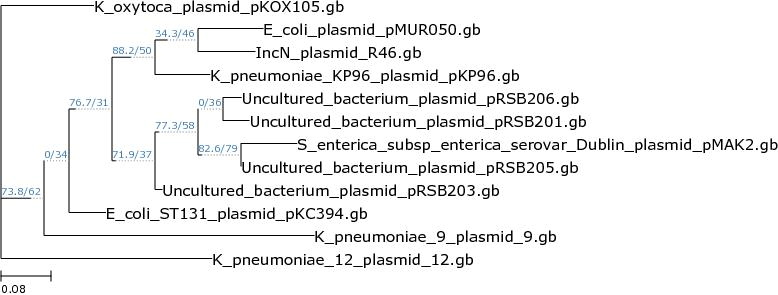
then the script calls program PARS from the PHYLIP suite to produce one or more alternative parsimony trees that capture the phylogeny implied in this matrix, adding the following lines to the produced output:
# parsimony results by PARS (PHYLIP suite, https://phylipweb.github.io/phylip/doc/pars.html):
# pangenome_phylip tree = sample_intersection/pangenome_matrix_t0.phylip.ph
# pangenome_phylip log = sample_intersection/pangenome_matrix_t0.phylip.log
The resulting tree (with extension .ph) is in Newick format
and is shown in Figure 10. Please note that such files might contain several equally parsimonious trees
separated by ';', one per line. In order to plot them, as in the next figure, it might be necessary to leave only one,
depending on the software used.
Both parsimony and ML trees with support estimates can be computed with script
estimate_pangenome_trees.sh from the GET_PHYLOMARKERS
pipeline.

|
|
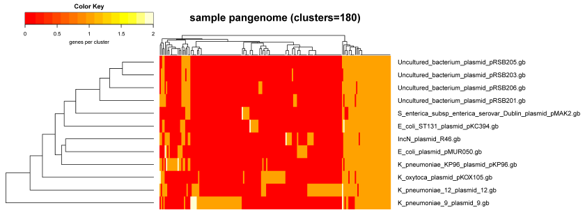
A complementary view of the same data con be obtained with script plot_matrix_heatmap.sh, which was called to produce Figure 12:
./plot_matrix_heatmap.sh -i sample_intersection/pangenome_matrix_t0.tab -o pdf \
  -r -H 8 -W 14 -m 28 -t "sample pangenome (clusters=180)" -k "genes per cluster"
|
Script parse_pangenome_matrix.pl can be used to analyze a pangenome matrix, such as that created in the previous section. It was primarily designed to identify genes present in a group A of species which are absent in another group B, but can also be used to find expansions/contractions of gene families. If you require the genes present/expanded in B with respect to A, just reverse them. Expanded clusters are defined as those where all A taxa contain more sequences than the maximum number of corresponding sequences in any taxa of group B.
We now review these features with the same plasmid set of previous sections, analyzing the pangenome matrix
produced by intersecting several cluster sets on section 4.9.1.
Let's say we are interested
in finding plasmid genes present in Klebsiella oxytoca which are not encoded in K.pneumoniae KP96.
In order to do this we first create a couple of text files to define sets A and B,
called A.txt and B.txt, which we place inside folder sample_plasmids_gbk.
The content of A and B files should be one line per species. In this example file
A.txt contains a single line:
K_oxytoca_plasmid_pKOX105.gb
As well as B.txt:
K_pneumoniae_KP96_plasmid_pKP96.gb
We can now execute the script as follows:
./parse_pangenome_matrix.pl -m sample_intersection/pangenome_matrix_t0.tab \
-A sample_plasmids_gbk/A.txt -B sample_plasmids_gbk/B.txt -g
The output should be:
# matrix contains 180 clusters and 12 taxa

# taxa included in group A = 1

# taxa included in group B = 1

# finding genes present in A which are absent in B ...
# file with genes present in set A and absent in B (21): [...]pangenome_matrix_t0__pangenes_list.txt
It can be seen that 21 genes were found to be present in A and absent in B.
In the case of pangenome matrices derived from GenBank files, as in this example, it is possible to
produce a map of these genes in the genomic context of any species included in A, which should be queried using
option -l. A valid syntax would be:
./parse_pangenome_matrix.pl -m sample_intersection/pangenome_matrix_t0.tab \
-A sample_plasmids_gbk/A.txt -B sample_plasmids_gbk/B.txt -g \
-p 'Klebsiella oxytoca KOX105'
By default, parse_pangenome_matrix.pl requires present genes to be present in all genomes of A and none of B.
However, as genomes might not be completelly annotated, it is possible to make these tests more flexible by controlling the cutoff for inclusion,
by using flag -P. For instance, the next command will require genes to be present only in 90% of A genomes and missing in 90% of B genomes:
./parse_pangenome_matrix.pl -m sample_intersection/pangenome_matrix_t0.tab \
-A sample_plasmids_gbk/A.txt -B sample_plasmids_gbk/B.txt -g -P 90
Note that the most flexible way of finding out genes absent in a set of genomes within a pangenome matrix is by using option -a,
which does not require an A list, rather a B list is sufficient. It is called as in the example:
./parse_pangenome_matrix.pl -m sample_intersection/pangenome_matrix_t0.tab \
-B sample_plasmids_gbk/B.txt -a
parse_pangenome_matrix.pl can also be employed to classify genes in these four compartments:
|
The script is invoked as follows:
./parse_pangenome_matrix.pl -m sample_intersection/pangenome_matrix_t0.tab -s
The output is as follows:
# matrix contains 180 clusters and 12 taxa

# cloud size: 124 list: sample_intersection/pangenome_matrix_t0__cloud_list.txt
# shell size: 23 list: sample_intersection/pangenome_matrix_t0__shell_list.txt
# soft core size: 33 list: sample_intersection/pangenome_matrix_t0__softcore_list.txt
# core size: 24 (included in soft core) list: sample_intersection/pangenome_matrix_t0__core_list.txt

# using default colors, defined in %COLORS

# globals controlling R plots: $YLIMRATIO=1.2

# shell bar plots: sample_intersection/pangenome_matrix_t0__shell.png , [...]shell.pdf
# shell circle plots: sample_intersection/pangenome_matrix_t0__shell_circle.png , [...]circle.pdf

# pan-genome size estimates (Snipen mixture model PMID:19691844): [...]shell_estimates.tab
Core.size Pan.size BIC LogLikelihood
2 components 24 193 1056.08217644576 -520.251652946544
3 components 23 370 583.140322949438 -278.587769347493
4 components 14 417 570.835786136617 -267.242544090193
5 components 13 703 579.364023427564 -266.313705884776
6 components 12 954 589.754861142051 -266.31616789113
7 components 13 808 600.134442088951 -266.313001513689
8 components 8 549 610.689900917556 -266.397774077102
9 components 0 572 621.283299953595 -266.501516744231
10 components 0 489 632.354613188809 -266.844216
Sample 24 180 NA NA
Apart from text files listing the cluster names that take part in each of the four compartments, two types of plots are
generated. The lenght of Y-axes in barplots can be controlled with global variable $YLIMRATIO,
as well as the colors used, by editing variable %RGBCOLORS.
Note that the output also includes estimates of the pan- and core-genome sizes as calculated by the binomial mixture model of Snipen and collaborators (PubMed=19691844). A simple interpretation is that as soon as likelihood converges then adding more components does not improve the mixture model. Please check that paper for a full explanation.
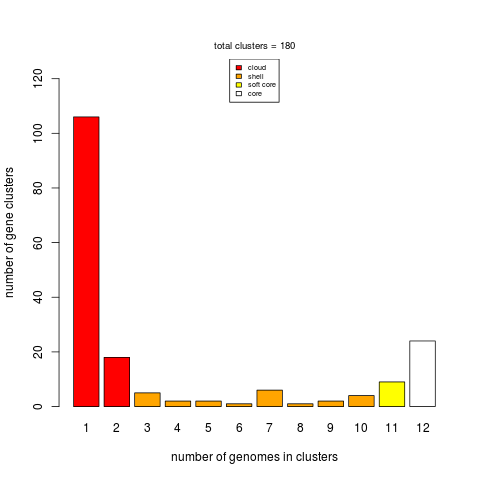
|
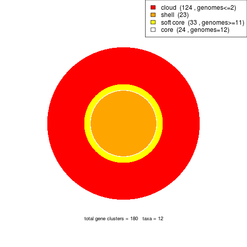
|
Optional flag -x can be added to the previous command in order to produce an intersection pangenome matrix:
./parse_pangenome_matrix.pl -m sample_intersection/pangenome_matrix_t0.tab -s -x
The output will now include the following:
# intersection pangenome matrix: pangenome_matrix_t0__intersection.tab
# mean %cluster intersection: 71.57
The reported mean value is the percentage of sequence clusters shared by any two input genomes. The TAB-separated file contains the number of clusters shared by all pairs of input genomes/sequence sets. Note that these clusters might contain several inparalogues of the same species:
intersection	E_coli_ST131_plasmid_pKC394.gb	E_coli_plasmid_pMUR050.gb	IncN_plasmid_R46.gb	...
E_coli_ST131_plasmid_pKC394.gb	51	39	39	...
E_coli_plasmid_pMUR050.gb	39	52	41	...
IncN_plasmid_R46.gb	39	41	58	...
...
The pioneer work of Tettelin and collaborators
(PubMed=16172379) unveiled
that bacterial genomes are dynamic containers that harbour essential genes and also
accessory elements, which might be unique to each community. get_homologues.pl can be used
to perform such genome composition analyses.
The rationale is to sample a set of genomes (present in the input folder) and keep adding genome
after genome keeping track of i) the novel genes added to the pool and ii) the genes that fall in
pre-existing clusters.
This sampling experiment can be done with any of the included 3 algorithms (please see Table 2),
by invoking option -c . For instance, we could try $ ./get_homologues.pl -d sample_buch_fasta -c:
[... same as first example ...]

# genome composition report (samples=10,permutations=24)
# genomic report parameters: MIN_PERSEQID_HOM=0 MIN_COVERAGE_HOM=20
# genome order:
# 0 Buch_aph_APS.faa
# 1 Buch_aph_Bp.faa
# 2 Buch_aph_Cc.faa
# 3 Buch_aphid_Sg.faa

## sample 0 (Buch_aph_APS.faa | 0,1,2,3,)
# adding Buch_aph_APS.faa: core=574 pan=574
[...]

# pan-genome (number of genes, can be plotted with plot_pancore_matrix.pl)
# file=sample_buch_fasta_homologues/pan_genome_algBDBH.tab
genomes	mean	stddev	|	samples
0	490	90	|	574	507	507	546	357	357	546	574	357	574
1	572	28	|	598	585	585	587	521	521	562	592	575	598
2	597	5	|	606	593	594	594	594	596	600	599	591	606
3	608	5	|	615	602	600	608	605	605	611	613	605	615

# core-genome (number of genes, can be plotted with plot_pancore_matrix.pl)
# file=sample_buch_fasta_homologues/core_genome_algBDBH.tab
genomes	mean	stddev	|	samples
0	490	90	|	574	507	507	546	357	357	546	574	357	574
1	420	82	|	466	466	466	523	324	324	317	523	324	466
2	327	36	|	319	319	434	315	310	315	313	318	309	319
3	310	4	|	313	313	313	311	304	304	311	313	304	313

[... same as first example ...]
|
As can be seen, the output now contains two data frames which summarize the
genome composition analysis done by sampling, which are also stored as tab-separated files.
These text files can be used to plot the core- and pan-genome, with help from
the accompanying script plot_pancore_matrix.pl. A suitable command would be:
./plot_pancore_matrix.pl -i sample_buch_fasta_homologues/core_genome_algBDBH.tab -f core_Tettelin
The script also supports the core function as modified by Willenbrock and
collaborators (PubMed=18088402),
as shown on the next figure in a more realistic set of 35 genomes. Both fits can be superimposed
by calling option -f core_both.
Besides standard core- and pan-genomes, it is possible to estimate the evolution of the soft core-genome,
which is a relaxed version of the core that considers genes found in a fraction (by default 0.95) of genomes, and thus accommodates
some annotation or assembly errors. This experiment can be done with either the OMCl or COGS algorithms
by invoking options -c -z. The resulting data file can be plotted the same way.
The genome composition analyses presented so far are actually random sampling experiments.
It is thus worth mentioning that the user can control the order in which genomes are sampled during
these simulations, by enforcing a list of genomes with option -I, already introduced in section 4.8,
or by setting the seed of the random number generator with option -R.
In the first case only one sampling is performed and therefore the standard deviation of the core and pan values is zero.
The second strategy ensures that sampling order is conserved in different program executions and thus allows merging CDS
core-genomes and non-coding genes (such as rRNAs) core-genomes computed separately over the same set of taxa, with help from
accompanying script add_pancore_matrices.pl.
Provided that Pfam domains have been annotated in advance (see section 4.5),
it is possible to calculate whether a set of clusters, for instance those that take part of the shell (see 4.9.3),
are enriched on a set of protein domains. To this end pfam_enrich.pl can be invoked as follows:
$ ./pfam_enrich.pl -d sample_plasmids_gbk_homologues/ \
  -c sample_plasmids_gbk_homologues/UnculturedbacteriumplasmidpRSB203_f0_0taxa_algOMCL_e0_ \
  -x sample_intersection/pangenome_matrix_t0__shell_list.txt -t less -p 1.0
There are several input data required for this kind analysis:
-d).
-c), obtained on earlier steps. These will be the 'control' set.
-x).
greater, two.sided or less, as in this example. The default is greater, which will test for Pfam
domains over-represented in 'experiment' clusters. Instead, greater tests for under-represented Pfam domains.
-r can be used to sample only sequences from a selected reference taxon.
-n should be called.
The output is as follows:
# parsing clusters...
# 756 sequences extracted from 193 clusters

# total experiment sequence ids = 148
# total control    sequence ids = 756

# parse_Pfam_freqs: set1 = 19 Pfams set2 = 103 Pfams

# fisher exact test type: 'less'
# multi-testing p-value adjustment: fdr
# adjusted p-value threshold: 1

# total annotated domains: experiment=19 control=144

#PfamID	counts(exp)	counts(ctr)	freq(exp)	freq(ctr)	p-value	p-value(adj)	description
PF00239	0	6	0.000e+00	4.167e-02	4.833e-01	9.860e-01	Resolvase, N terminal domain
PF01526	0	6	0.000e+00	4.167e-02	4.833e-01	9.860e-01	Tn3 transposase DDE domain
PF02796	0	3	0.000e+00	2.083e-02	6.928e-01	9.860e-01	Helix-turn-helix domain of resolvase
PF12681	0	3	0.000e+00	2.083e-02	6.928e-01	9.860e-01	Glyoxalase-like domain
[...]
If we recall for a moment the example GenBank files analyzed on section 4.4 we can
demonstrate how to calculate average identity matrices, which can then be used to compare genome members of
a pangenome. To do so we will add a few flags to the previous command, in addition to flag -A, which specifically asks for an identity matrix to be calculated:
$ ./get_homologues.pl -d sample_plasmids_gbk -A -t 0 -M
Similarly, flag -P can be invoked to produce matrices of percentage of conserved proteins.
This will produce the following output:
[...]
# number_of_clusters = 193
# cluster_list = [...]/UnculturedbacteriumplasmidpRSB203_f0_0taxa_algOMCL_e0_.cluster_list
# cluster_directory = [...]/UnculturedbacteriumplasmidpRSB203_f0_0taxa_algOMCL_e0_

# average_identity_matrix_file =
# [...]/UnculturedbacteriumplasmidpRSB203_f0_0taxa_algOMCL_e0_Avg_identity.tab
# NOTE: matrix computed on blastp results
Note that on this example the produced identity matrix was calculated with the BLASTP scores among protein sequences included on the resulting clusters (193). If average nucleotide identities are desired the command must be modified to:
$ ./get_homologues.pl -d sample_plasmids_gbk -a 'CDS' -A -t 0 -M
Such matrices can then be used to calculate heatmaps and dendrograms that capture how similar the coding sequences are among genomes. An example of this would be:
cd sample_plasmids_gbk_homologues
../plot_matrix_heatmap.sh -i EcoliST131plasmidpKC394_f0_0taxa_CDS_algOMCL_e0_Avg_identity.tab \
  -d 2 -t "CDS ANI matrix with 2 decimals"
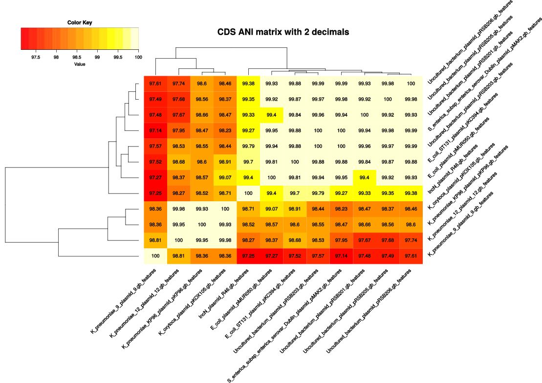
|
A
After running get_homologues with almost any set of parameters, you will always end up with a lot of BLAST files
of all-against-all involved taxa. The accompanying script check_BDBHs.pl can help you find out which are the best BLAST
hits of any sequence that might interest you.
First, as cluster names are not always informative, you'll need to find out the internal identifier used by the software to handle your
target sequence. For instance, we might want to investigate protein CspE among our 4 Buchnera taxa. The command to achieve this would be:
$ ./check_BDBHs.pl -d sample_buch_fasta_homologues -g -i CspE:
And we obtain:
# Sequences containing label CspE:

1360,Buch_aph_Cc.faa,gi|116515229|ref|YP_802858.1| CspE [Buchnera aphidicola str. Cc (Cinara cedri)]
Now that we know the identifier (1360), we can check its best hits:
$ ./check_BDBHs.pl -d sample_buch_fasta_homologues -i 1360
Output contains the identifiers of best hits in both directions, their bit-scores, E-values, alignment %coverages and annotated Pfam protein domains when available:
# query = 1360
# query fullname = gi|116515229|ref|YP_802858.1| CspE [Buchnera aphidicola str. Cc (Cinara cedri)]

# list of bidirectional best-hits:
dir	query	  sbjct	  bits	  Eval	  %ident	cover	  Pfam	   annotation
:						                                             [Buch_aph_APS.faa]
>	   1360	    467	   136	 4e-42	    97.1	100.0	  NA	     gi|15617086|..cold shock protein E

<	    467	   1360	   136	 4e-42	    97.1	100.0	  NA
:						                                             [Buch_aph_Bp.faa]
>	   1360	    972	   135	 1e-41	    95.7	100.0	  NA	     gi|27904911|..cold shock protein E

<	    972	   1360	   135	 1e-41	    95.7	100.0	  NA
:						                                             [Buch_aphid_Sg.faa]
>	   1360	   1883	   136	 4e-42	    97.1	100.0	  NA	     gi|21672738|..cold shock protein E

<	   1883	   1360	   136	 4e-42	    97.1	100.0	  NA
If previous get_homologues jobs included the calculation of Pfam domains, then option -D can be added to
produce a richer report, that now includes the identifiers of Pfam domains such as
PF00313, sorted on their position along the sequence:
dir	query	  sbjct	  bits	  Eval	  %ident	cover	  Pfam	   annotation
:						                                             [Buch_aph_APS.faa]
>	   1360	    467	   136	 4e-42	    97.1	100.0	  PF00313,	     gi|15617086|..cold shock protein E

<	    467	   1360	   136	 4e-42	    97.1	100.0	  PF00313,
...
Note that this script works by parsing files all.p2o.csv and all.bpo, which are created at run-time by
get_homologues in folder tmp/ within the results directory.
These are text files that can be inspected with help from any text editor.
File HOWTOTettelin is a shell script which performs typical uses of get_homologues.pl,
including jobs that require Pfam. This script can be
executed with: $ ./HOWTOTettelin
The first task carried out by the script is to download the same GenBank files used in the landmark work of Tettelin
and collaborators (PubMed=16172379); afterwards
several analyses are sequentially undertaken:
# 1.0) optionally download genomes in GenBank format from NCBI FTP site
cd test_Streptococcus
../download_genomes_ncbi.pl test_Streptococcus_download_list.txt
cd ..

# 1.1) run BLAST jobs with 4 CPU cores and optionally HMMER
./get_homologues.pl -d test_Streptococcus/ -n 4 -o
./get_homologues.pl -d test_Streptococcus/ -n 4 -D -o

# 1.2) calculate core-genomes with all BDBH, OMCL & COG algorithms
./get_homologues.pl -d test_Streptococcus/
./get_homologues.pl -d test_Streptococcus/ -M
./get_homologues.pl -d test_Streptococcus/ -G
./get_homologues.pl -d test_Streptococcus/ -M -D

# 1.3) calculate consensus core-genome with syntenic genes
./compare_clusters.pl -s -n -o test_Streptococcus_intersection -d \
test_Streptococcus_homologues/S_f0_alltaxa_algCOG_e0_,\
test_Streptococcus_homologues/S_f0_alltaxa_algOMCL_e0_,\
test_Streptococcus_homologues/S_f0_alltaxa_algBDBH_e0_

# 1.4) calculate core-genome with coverage and identity as in the Tettelin paper (cover=50%,%ID=50)
./get_homologues.pl -d test_Streptococcus/ -M -C 50 -S 50

# 1.6) calculate core intergenic clusters
./get_homologues.pl -d test_Streptococcus/ -g

# 1.7) estimate and plot core- and pangenome sizes with all BDBH, OMCL & COG algorithms
./get_homologues.pl -d test_Streptococcus/ -c
./get_homologues.pl -d test_Streptococcus/ -M -c
./get_homologues.pl -d test_Streptococcus/ -G -c

# 2.1) calculate pan-genome with OMCL & COG algorithms
./get_homologues.pl -d test_Streptococcus/ -M -t 0
./get_homologues.pl -d test_Streptococcus/ -G -t 0

# 2.2) build consensus pangenomic matrix
./compare_clusters.pl -d test_Streptococcus_homologues/S_f0_0taxa_algCOG_e0_,\
test_Streptococcus_homologues/S_f0_0taxa_algOMCL_e0_ -m -T -o test_Streptococcus_intersection

# 2.3) plot pangenomic compartments and estimate core- and pan-genome size with mixture models
./parse_pangenome_matrix.pl -m test_Streptococcus_intersection/pangenome_matrix_t0.tab -s

# 2.4) check accesory genes present in A genomes and absent in B
./parse_pangenome_matrix.pl -m test_Streptococcus_intersection/pangenome_matrix_t0.tab \
	-A test_Streptococcus/A.list -B test_Streptococcus/B.list -g -e
Readers looking for a fully worked out example, including a comprehensive interpretation of results, can read our book chapter "Robust Identification of Orthologues and Paralogues for Microbial Pan-Genomics Using GET_HOMOLOGUES: A Case Study of pIncAC Plasmids" (PubMed=25343868).
Please see also
Not really. It can be run on a single machine, but if you have say, more than 10 microbial genomes, the required all-against-all BLAST jobs
would take some time to complete, depending on your hardware. If this is your case we recommend setting option -n to the number
of cores of your processor,
as this way BLAST/HMMER jobs will be split and sent to different jobs and the required computing time proportionally reduced.
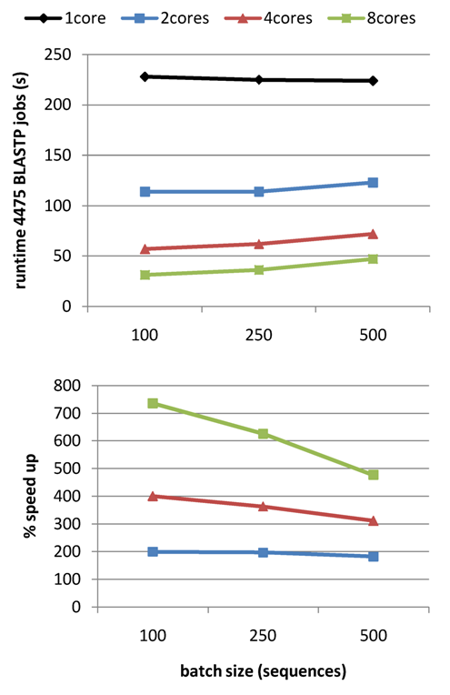
|
Cluster jobs are submitted by invoking option -m cluster
Detailed configuration instructions for gridengine, LSF and Slurm job managers are on section 2.3.
You might need to create a file HPC.conf to match your local environment. For instance,
in a gridengine/SGE system you might get the following error:
# running BLAST searches ...
Unable to run job: You have to specify a queue, with the '-q' option to qsub.
Exiting.
[...]
This usually means that farm jobs inside get_homologues.pl need a target queue in the cluster.
Please find out the name of the right queue for your jobs, perhaps something as simple as such as -q default,
and edit the relevant line in HPC.conf:
QARGS -q default
As Perl is not installed by default on Windows, not BerkeleyDB is easily installed there, we haven't ported this software to these systems. However, with some work, you could probably set up a windows machine to run get_homologues.pl and most of its dependencies. Nevertheless, we have tested the package only on Linux and macOSX systems, and currently the only supported option for Windows users is the Docker container at https://hub.docker.com/r/csicunam/get_homologues
This depends directly on the size and number of the genomes to be analyzed.
A recent benchmark with 71 Mycobacterium genomes and 280k sequences yielded a RAM usage of just over 3700 MB,
confirming that versions 2.* have a much reduced memory footprint (see Figure 20, in the original
benchmark up to 40 microbial genomes could be analyzed on a 8Gb RAM Linux box).
Moreover, as mentioned in section 3.4, the -s flag option reduces the memory footprint of your
get_homologues up to 20-fold, allowing running large jobs in machines with small RAM resources.
Therefore, if you are running a large job that fails to finish succesfully, the most common
explanation would be that it was killed by the operating system for taking too much memory. In those cases it is
advisable to re-run the same job with the -s flag.
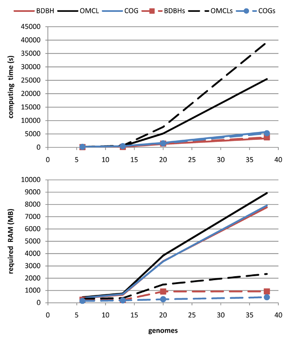
|
After evolving parts of the original code base, and fixing some bugs (see CHANGES.txt), both get_homologues.pl and get_homologues-est.pl have significantly improved their performance, as can be seen in the figure, which combines data from the original benchmark and new data generated after v2 was in place.
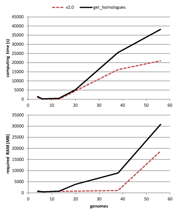
|
When solving problems related with submitting jobs to the cluster it is
necessary to check the generated .queue files, which capture any errors that might occur during job submission.
If you check one of these files an find a message such as
blast: error while loading shared libraries: libbz2.so.1: cannot open shared object file
this means that some cluster nodes will require the installation of 32-bit compatibility library libbz2.so.1,
which can be done with root privileges typing this command from your cluster master node:
rocks run host compute "yum -y install bzip2-libs.i386"
Another solution would be to use BLAST binaries native to your cluster architecture, as explained in section 2.2.
In the v2 code family BLAST parsing evolved to capture -outfmt 6 'qseqid sseqid pident length qlen slen qstart qend sstart send evalue bitscore'. However, the original code base was capturing different data columns and this implies that old BLAST results from previous releases won't work anymore.
Option -S 1 means that two sequences can be considered orthologues or inparalogues with any sequence identity,
provided that
![]() and alignment coverage is sufficient (
and alignment coverage is sufficient (-C). This can be useful when
comparing very divergent genomes/proteomes, where orthologues can be distant in terms of sequence.
If a reciprocal hit between genomes A and B is, say 30% identical, still it is a likely orthologue.
It could of course be a false positive, and that's why you need to know, perhaps by using -A, the average identity
among proteins in those genomes, and ultimately a gene phylogenetic tree, including species A, B and others to compare
to the species tree.
-o is good for?
This option is useful in situations like the following: you have access to a compute cluster with modern compute nodes (64bit cores and a good amount of memory),
but the master computer is an old, 32bit machine with limited RAM (say 1GB or less). Under such a setting, it would be convenient to distribute the first steps
of the pipeline (all against all BLAST jobs) on the cluster using options -o -m cluster. The downstream parsing of the BLAST results, which is
memory-consuming, could then be executed logged in from one of the more powerful compute nodes or from a powerful server.
-o, to log into three different compute nodes
and execute the downstream pipeline on each node for a different clustering algorithm (i.e. BDBHs, COG and OMCL)?
No, as each get_homologues.pl job requires exclusive access to the data directory and prevents other jobs to access it simultaneously.
Of course, as this option enforces the program to sample once the list of genomes in the implicit order of the list. The fitting of pan-/core-genome functions will be affected as there will be less points to do the noon-linear fitting.
This parameter captures the concept of BLAST neighborhood explained in PubMed=18475320, and is calculated as a a positive Pearson correlation coefficient. In this context, sequences A and B should have a similar list of BLAST matches if they truly are orthologues. This parameter is by default set to 0, so it takes no effect. As its values approaches to 1, it gets more difficult to call bidirectional best hits, as they will be required to have very similar lists of BLAST hits.
-t option?
You should use -t 0 (zero) when you need to get all clusters of homologous sequences.
This will generate files containing 2 or more homologous sequences from one or more taxa.
By default, get_homologues.pl sets t=numberOfTaxa, that is, it will provide the user with clusters of homologous sequences
that contain at least one sequence from each taxon. Note that singleton clusters (just one sequence per organism) will be produced
if combined with option -e, which excludes clusters containing inparalogues. In this later case, the resulting clusters will
contain only single copy genes from each taxon, i.e. the orthologues. This is convenient if you want to use resulting gene families
to do for example genome-level phylogenetic analyses using only the repertoire of orthologous single copy genes. Note, however, that
such clusters are not suitable for pangenome analyses. For such analyses, instead, please use auxiliary script compare_clusters.pl
with the set of clusters obtained with -t 0.
Thoroughly annotated genomes (see for example the GenBank file for Escherichia coli K12 MG1655:
Escherichia_coli_K_12_substr__MG1655_uid225.gbk)
have many features, incluing ribosomal rRNAs, intergenic spacers, tRNAas, 'mat_peptide', 'repeat_region', and miscellaneous features,
noted as 'misc_feature',
in the corresponding GenBank files. Miscellaneous features report on diverse things such as cryptic prophages, the target sites of resolvases involved
in replicon replication, and many more "miscellaneous" features. Note that there is great heterogeneity both in the format and detail of annotating
genome features. By default, get_homologues.pl will extract only the 'CDS' feature (i.e. the sequences for protein-coding sequences) from the
GenBank file. By using option -a the user can select which features to parse, such as 'tRNA' or 'rRNA'.
The original OrthoMCL paper (PubMed=12952885) explains it: "[...] changing the inflation index affects cluster tightness: Lower inflation values result in the inclusion of more sequences in fewer groups, whereas increasing the inflation index fragments clusters and reduces the number of sequences included". In our benchmarks with bacterial genomes this parameter shows a very modest, negligible effect.
If you still conserve the original input folder with FASTA or GenBank sequence files and the results _homologues directory,
both contained in the same directory, all you will have to do is to copy the new sequence files to the input folder and re-run
get_homologues.pl. This will ensure that only new required BLAST/PFam searches are completed, conserving the previous results as much
as possible.
Cluster files are named using gene names from the reference genome, or from the first included genome otherwise.
If a given genome R is selected with option -r then gene names from R will be used preferably.
It is possible to change the way clusters are named by editing subroutine extract_gene_name in file lib/phyTools.pm.
The most obvious effect is that any resulting clusters will now be named according to gene names of the new reference genome. A more subtle consequence for BDBH jobs is that now all genomes are compared to this reference, see figure 3, and this will change the order in which bidirectional best hits are computed.
In this case the genome with the least number of genes/features will be taken as the reference, and resulting sequence clusters will be named according to gene names of this reference genome, which might not be the best annotated genome in your set. For this reason it is often a good idea to set as reference genome one with a good annotation, for instance the species or strain described in RefSeq.
Option -b is only suited for core-genome calculation, not pangenome. If this is really the desired task, the genome with the least number
of annotated genes should be used as a reference, which is what the program would do by default, or else the best-annotated among small genomes.
However, note that this sort of core-genome calculation is most sensitive to missing genes, usually due to poor automatic annotations, which is
why compiling a pangenome matrix is recommended when possible (see Section 4.9.1), so that a more robust soft-core can be estimated.
The reason is that BDBH uses a single reference genome and thus by definition cannot track genes not present in the reference. Therefore, pangenome matrices produced by the BDBH algorithm would be incomplete, considering only clusters including genes from the reference genome. For this reason BDBH is adequate for core-genome calculation, but not for pan-genomes.
Within lib/marfil_homology.pm there is a global variable $BLAST_DB_SIZE set to 100_000_000 for that purpose.
That value is the fixed effective search space during BLAST searches so that any resulting E-values are comparable, even across experiments
or algorithm (BDBH, OMCL, COGS).
inparalogues_Buch_aph_APS.faa. Could you explain about the files or a method to extract the information?
According to our working definition, all sequences grouped together in the same .faa/.fna cluster are likely orthologues, although you should always keep in mind that orthology is an evolutionary concept and therefore sequence-based approaches such as those in get_homologues.pl are simpler approximations. What is different with inparalogues? They are supposed to be duplicated genes that appeared after species separation, and therefore their orthology relationships are many-to-one or many-to-many. Inparalogues are easy to spot in clusters produced by get_homologues.pl because they are 2+ sequences from the same genome in the same cluster cluster. If you wish to know which inparalogue is most similar to an orthologous gene the best option is to run check_BDBHs.pl, which is explained on Section 4.9.7.
BLAST parameter -max_target_seqs is set to the number of sequences of the query proteome, which usually is a large number
that ensures all good quality hits are recovered. Read more here.
Although get_homologues.pl scripts explicitily flush output buffers (set with $|=1),
users can occasionally experience buffering problems when writing to slow, external hard drives, as output files are often very large.
Such problems have been reported when calling -G option, which in turn invokes subroutine find_COGs and calls several
external binaries, whose buffers cannot be flushed from the scripts. If that happens to you please consider increasing the sleep time
in that sub, which by default is 10 seconds.
It is possible to experimentally normalize the scores using the script here. However, our tests suggest this might cause unexpected consequences and for that reason this is not done by default.
Pancore matrices contain estimates of core- and pan-genomes and they are produced by get_homologues.pl with option -c.
These files take names such as pan_genome_algBDBH_C75.tab, which record the algorithm employed, and are generated by random-sampling genomes.
Sampling can be controlled and reproduced by using the same random-number generator seed (see section -R in Section 3.4).
Such files can be used to render plots (and fitted functions) with script plot_pancore_matrix.pl, as shown in Section 4.9.4.
Instead, pangenome matrices are generated by accessory script compare_clusters.pl, and contain information about what which genomes contain sequences
from gene clusters, with no sampling involved (see Section 4.9.1).
They take names such as pangenome_matrix_t0.tab.
Yes, no problem. The script will generate the intersection_t0.cluster_list , pangenome_matrix_t0.phylip and pangenome_matrix_t0.tab
files based on the clusters found by the chosen algorithm. The only thing you won't find in the directory are Venn diagrams, since at least 2 cluster sets
(generated by 2 algorithms) are required to compute them.
When provided with the output directories holding the clusters generated by 2 or 3 algorithms, the script will select only those clusters that contain exactly the same sequences in each of the clusters. This may be valuable for example if the user is interested in defining a very robust core genome set, containing only those families with exactly the same members, independently of the chosen algorithm. However, it is possible that several otherwise important families get lost for downstream analyses, such as presence-absence analyses of gene families in pairs of lineages, which can be done with parse_pangenome_matrix.pl.
BDBH results cannot be used for pangenome analysis, but you could re-run the software with the same 25 input genomes, now adding -t 0 -M for OMCL,
probably the best choice for such an analysis. This will re-use all blast results previously calculated and resume until OMCL analysis is completed.
Usually core sets produced by BDBH, COGS and OCML are very similar. Therefore, most of your previously tested core genes should also be picked up
by OCML on this second run, and presumably you could now proceed to pangenome analysis.
You have calculated 3 core-genomes from 3 different sets of strains and now you want to know the subset of core-genes present in all individual core-genomes. If you check compare_clusters.pl option you'll see that it says "by default cluster dirs are expected to be derived from the same taxa", which is exactly what's failing in your examples. If you want to find common core-clusters present if all 3 sets and also those shared by only some of the taxa I guess you should build a pangenome matrix by running get_homologues.pl with all strains together with option -t 0. The matrix itself will give you the clusters present/absent in all and some of the strains, which I guess is what you need. The script parse_pangenome_matrix.pl can read this matrix and further help you identify these clusters.
Option -r can be used to compare a list of core genes from a single genome G,
that is, with clusters containing only sequences from G, to clusters of a larger group of taxa (A,B,C,...,G) that includes G.
compare_cluster.pls -T cannot be opened by MEGA
Program pars from the PHYLIP suite
often produces several alternative parsimony trees contained in the
pangenome_matrix_t0.phylip.ph file,
one per line. Some phylogeny programs, such as
MEGA, require splitting these trees in separate files in order to properly read and plot them.
When a command such as ./parse_pangenome_matrix.pl -m pangenome_matrix_t0.tab -A A.txt -B B.txt -g is invoked,
the passed A & B files must contain taxon names matching exactly those of corresponding input files, including the extension. Instead of
a list such as:
taxonA
taxonB_001
...
taxonZ244
the list should be:
taxonA.faa
taxonB_001.faa
...
taxonZ244.faa
-C 75 -S 70 does not match the pangenome size estimated with option -c
The reason for these discrepancies is that they are fundamentally different analyses.
While the default runmode simply groups sequences trying to put in the same clusters orthologues and inparalogues,
a genome composition analysis performs a simulation in order to estimate how many novel sequences are added by
genomes sampled in random order. In terms of code, there are a couple of key global variables set in
lib/marfil_homology.pm, lines 130-131, which control how a gene is compared to previously processed pangenome
genes in order to call it novel:
$MIN_PERSEQID_HOM = 0;
$MIN_COVERAGE_HOM = 20;
The first variable is set by default to 0, meaning that there is no %identity limitation to call homologues.
The second is set to 20, which means that any sequence matching a previous gene with
![]() will be considered homologous and thus won't be considered new. As you can see these are very stringent values.
will be considered homologous and thus won't be considered new. As you can see these are very stringent values.
Now, in your settings, you might want to change these values. For instance, Tettelin in their landmark work used values of 50 and 50
(PubMed=16172379),
which means that protein sequences with
![]() and
and
![]() to previous genes will be called homologues,
and therefore won't be accumulated to the growing pangenome. In other words, you should tweak these variables to your particular settings.
to previous genes will be called homologues,
and therefore won't be accumulated to the growing pangenome. In other words, you should tweak these variables to your particular settings.
The two trees are equally parsimonious, that is, have the same parsimony score but different topologies. One possibility to combine them into one topology is to compute either the majority rule consensus (mjr) tree, for example with consense from the PHYLIP package, or represent a network consensus with a program such as splitstree.
Regarding the bootstrapping, you could write some R code (or in any other language) to randomly sample the columns
in the pangenome matrix with replacement to construct a new, bootstrapped matrix with the same number of columns
as the original one. You should generate 100 or 500 of these matrices and then run pars on each one of them.
Then run consense to obtain the mjr consensus tree and associated split frequencies (bootstrap support values for each bipartition).
An easy way of achieving this would be with R's boot
package
(see example).
Another option is to call seqboot from the PHYLIP package to generate N bootstrap pseudo-replicates of the matrix.
Rename the resulting file as infile and call pars to read the file, using the option m no_of_pseudoreplicates
to run the standard (Fitch) parsimony analysis on each of the bootstraped matrices. PHYLIP pars will generate an outtree file
containing as many trees as bootstraped matrices found in infile. Rename outtree to intree and call consense to generate the
default majority rule consensus tree. This tree is only a cladogram (only topology, no branch lengths).
The node labels correspond to the number of bootstrap pseudoreplicates in which that particular bipartition was found.
Let's say you have 20 genomes, then 95% of them are exaclty 19 taxa, which is the minimum occupancy that defines soft-core clusters
(see global variable $SOFTCOREFRACTION). You should then compute the ANI matrix as follows:
./get_homologues.pl -d your_data -a 'CDS' -A -M -t 19
And then plot the resulting matrix with script hcluster_pangenome_matrix.sh.
The difference in the topologies of the NJ trees and the row-dendrogram of the heatmaps differ because the heatmaps are ordered bi-dimensionally. That is, the heatmap plot shows only the row-dendrogram, but the matrix is ordered also by columns. The NJ tree is computed from the distance matrix that you indicate the program to calculate for you (ward.D2 is the default).
compare_clusters.pl -T?
The PARS program from the PHYLIP suite reconstructs the pan-genome phylogeny using the parsimony optimality criterion. As such, each column in the input pangenome matrix is considered an independent character, and character state changes (within columns) are considered to represent a single evolutionary event (have a weight of 1) in standard parsimony. As can be read in its documentation, the algorithm used for estimating branch lengths averages the number of reconstructed changes of state over all sites, over all possible most parsimonious placements of the changes of state among branches. Note that it does not correct in any way for multiple changes that overlay each other. Therefore, the scale that you find at the bottom of the tree corresponds to average number of state transitions or steps, as estimated under the standard or Fitch parsimony criterion. It is hence the parsimony estimate of the "distance" in number of steps (differences in cluster composition, in our case). Given that it is an average, the branch lengths (number of steps) are real numbers, not integers, as one might expect.
If you did your analysis requesting cluster of all occupancies (-t 0) then you can get what you want in two steps.
First, you must produce a pangenome matrix with compare_clusters -d ... -m. Now it is possible to request an intersection
pangenome matrix (pangenome_matrix_t0__intersection.tab) which contains the number of sequence clusters shared by
any two pairs of genomes with parse_pangenome_matrix.pl -m pangenome_matrix_t0.tab -s -x.
Note that these clusters might contain several inparalogues of the same species.
Please refer to manual_get_homologues-est.pdf for an example application of this script.
Please refer to manual_get_homologues-est.pdf for an example application of this script.
We recommend script estimate_pangenome_trees.sh from the GET_PHYLOMARKERS
pipeline. Another alternative is to use the .fasta version of the pangenome matrix produced by script ./compare_clusters.pl -m ,
next to the .tab and .phy files.
This FASTA file can be analyzed with ML software such as IQ-TREE
(PubMed=25371430) both online or in the terminal with a command such as:
path_to_iqtree -s pangenome_matrix_t0.fasta -st BIN -m TEST -bb 1000 -alrt 1000
This will produce an optimal ML tree after selecting a binary substitution model with both bootstrap and aLRT support values.
Note that GET_PHYLOMARKERS will stop if two input genomes have the same name and strain in the FASTA files produced by get_homologues; if that happens you might need to edit the headers of those files. This is one way this can be done:
for f in *.faa; do perl -pi.bak -e 's/\|\|Bacillus1.gbk/|1|Bacillus1.gbk/g' $f; done
for f in *.faa; do perl -pi.bak -e 's/\|\|Bacillus2.gbk/|2|Bacillus2.gbk/g' $f; done
|
get_homologues.pl is designed, created and maintained at the Laboratory of Computational Biology at EstaciĂłn Experimental de Aula Dei-CSIC in Zaragoza (Spain) and at the Center for Genomic Sciences of Universidad Nacional AutĂłnoma de MĂ©xico (CCG/UNAM).
The code was written mostly by Bruno Contreras-Moreira and Pablo Vinuesa, but it also includes
code and binaries from OrthoMCL v1.4
(algorithm OMCL, -M),
COGtriangles v2.1
(algorithm COGS, -G),
NCBI Blast+, MVIEW
and BioPerl 1.5.2.
Other contributors: Carlos P Cantalapiedra, Alvaro Rodriguez del Rio, Ruben Sancho, Roland Wilhelm,
David A Wilkinson.
We ask the reader to cite the main references describing the get_homologues software,
and also the original papers describing the included algorithms and databases, accordingly:
If you use the accompanying scripts the following references should also be cited:
This document was generated using the LaTeX2HTML translator Version 2019.2 (Released June 5, 2019)
The command line arguments were:
latex2html manual -no_antialias_text -split 0 -dir manual -no_navigation -show_section_numbers
The translation was initiated on 2026-01-08