Preparation, selection and mapping of climate variables
26/Sep/2018
This document describes how climate data (1981-2010), compiled by R Serrano and S Beguería, and analyzed also by B Contreras Moreira, were processed in order to carry out Genome–Environment Association (GEA) in combination with barley SNPs.
Inspecting the raw data
The original data file was renamed to barley_climate_updated.tsv](raw/barley_climate_updated.tsv) and lines SBCC142-5 manually commented out, leaving only mainland, Iberian barleys. Note that SBCC138 was also left out as suggested by AM Casas due to uncertainty in genotype data. In addition, note that line SBCC036 lacks data for variables et0_spr, bal_aut, bal_win, bal_jun, bal_mar_apr_may, and was thus excluded from the climate-complete dataset. The following variables are currently included:
| var | full name |
|---|---|
| \(\mbox{pcp}\) | average cumulative precipitation |
| \(\mbox{pcp}_{p10}\) | average 10th percentile of cumulative precipitation |
| \(\mbox{tmed}\) | average daily mean temperature |
| \(\mbox{tmax}\) | average daily max temperature |
| \(\mbox{tmin}\) | average daily min temperature |
| \(\mbox{tamp}\) | average daily thermal amplitude (Celsius) |
| \(\mbox{verna}\) | average potential vernalization (days) |
| \(\mbox{verna}_n\) | average number of days since 15th November to reach \(n=(10,20,30,40)\) vernalization days |
| \(\mbox{frost}\) | average number of frost days |
| \(\mbox{pfrost}_{01}\) | average first day in the year where \(p(\mbox{tmin}<0) \leq 0.10\) |
| \(\mbox{et0}\) | average potential evapotranspiration, according to FAO56 Penman-Monteith |
| \(\mbox{bal}\) | climatic water balance (\(\mbox{pcp}\) - \(\mbox{et0}\)) average potential evapotranspiration, according to FAO56 Penman-Monteith |
| \(\mbox{dummy}\) | random data with some spatial coherence |
Altitude/elevation data are stored on file SBCC_altitude.tsv.
For each variable with the exception of \(\mbox{pfrost}_{01}\) monthly, seasonal and annual averages are given. Monthly values are signaled with subscripts _01 to _12, while seasonal and annual values are denoted by the subscripts _spr, _aut, _win and _annual. Summer aggregates and months between July and October are not expected to have any influence on barley cultivars, hence they were excluded on further analyses.
Dummy climate variables were simulated as explained in this blog post by S Beguería.
# read raw data (landraces SBCC138,142-5 previously excluded)
rawdata <- read.table(file="raw/barley_climate_updated.tsv", header=TRUE, sep="\t")
# read altitude (skipping SBCC138,142-5)
altitude <- read.table(file="raw/SBCC_altitude.tsv",header=T)
rawdata <- merge(rawdata, altitude, by="id")
# fix var names
# #month is replaced by 3-letter string
# vernalization days are made explicit
climvarnames = colnames(rawdata)
climvarnames = gsub("pfrost_01", "pfrost", climvarnames)
climvarnames = gsub("verna_d_01", "verna_10d", climvarnames)
climvarnames = gsub("verna_d_02", "verna_20d", climvarnames)
climvarnames = gsub("verna_d_03", "verna_30d", climvarnames)
climvarnames = gsub("verna_d_04", "verna_40d", climvarnames)
climvarnames = gsub("dummy_", "dummy", climvarnames)
climvarnames = gsub("_01$", "_jan", climvarnames)
climvarnames = gsub("_02$", "_feb", climvarnames)
climvarnames = gsub("_03$", "_mar", climvarnames)
climvarnames = gsub("_04$", "_apr", climvarnames)
climvarnames = gsub("_05$", "_may", climvarnames)
climvarnames = gsub("_06$", "_jun", climvarnames)
climvarnames = gsub("_07$", "_jul", climvarnames)
climvarnames = gsub("_08$", "_aug", climvarnames)
climvarnames = gsub("_09$", "_sep", climvarnames)
climvarnames = gsub("_10$", "_oct", climvarnames)
climvarnames = gsub("_11$", "_nov", climvarnames)
climvarnames = gsub("_12$", "_dec", climvarnames)
climvarnames = gsub("dummy", "dummy_", climvarnames)
colnames(rawdata) = climvarnames
# exclude months between harvest and planting
# exclude unsed percentile10 vars
alldummies <- rawdata[,grep("dummy|id",colnames(rawdata),perl=T)] # before removing summer months
w <- grep('sum|jul|aug|sep|oct|_p10_', names(rawdata), perl=TRUE)
rawdata <- rawdata[,-w]
# separate dummy and climate* variables
dummydata <- rawdata[,grep("dummy|id",colnames(rawdata),perl=T)]
geodata <- rawdata[,grep("utmx|utmy|altitude|id",colnames(rawdata),perl=T)]
climdata <- rawdata[,grep("dummy|utm",colnames(rawdata),perl=T,invert=T)]
pcp <- climdata[,grep("pcp",colnames(climdata))]
tmed <- climdata[,grep("tmed",colnames(climdata))]
tmax <- climdata[,grep("tmax",colnames(climdata))]
tmin <- climdata[,grep("tmin",colnames(climdata))]
amp_termica <- climdata[,grep("tamp",colnames(climdata))]
heladas <- climdata[,grep("frost|probab",colnames(climdata))]
vernal <- climdata[,grep("verna",colnames(climdata))]
drought <- climdata[,grep("et0|bal",colnames(climdata))]Exploratory analysis
The climate data was inspected by calculating correlations (see sample plot) and histograms:
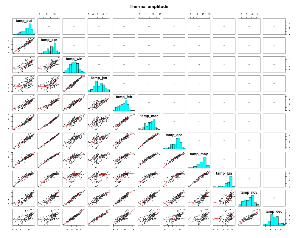
# example of auto-correlations (both in report and file)
panel.hist <- function(x, ...) {
usr <- par("usr"); on.exit(par(usr))
par(usr = c(usr[1:2], 0, 1.5) )
h <- hist(x, plot=FALSE)
breaks <- h$breaks; nB <- length(breaks)
y <- h$counts; y <- y/max(y)
rect(breaks[-nB], 0, breaks[-1], y, col = "cyan", ...)
}
panel.cor <- function(x, y, digits = 2, prefix = "", cex.cor, ...) {
usr <- par("usr"); on.exit(par(usr))
par(usr = c(0, 1, 0, 1))
r <- abs(cor(x, y, use="pairwise.complete.obs"))
txt <- format(c(r, 0.123456789), digits = digits)[1]
txt <- paste0(prefix, txt)
if(missing(cex.cor)) cex.cor <- 0.8/strwidth(txt)
text(0.5, 0.5, txt, cex=cex.cor*r)
}
png("plots/amp_termica.png",height=800,width=1000)
aux <- amp_termica
names(aux) <- gsub('amp_termica_','',names(amp_termica))
pairs(aux, panel=panel.smooth, pch=21, cex=0.5, bg='light blue',
diag.panel=panel.hist, upper.panel=panel.cor,
cex.labels=1.5, font.labels=2, #cex.cor=1.5,
main='Thermal amplitude')
dev.off()png
2 # histograms to check what they look like
par(mfrow=c(5,3), mar=c(3,3,3,2)+0.1)
hist(geodata$utmx,main="longitude (UTM)")
hist(geodata$utmy,main="latitude (UTM)")
hist(geodata$altitude,main="elevation")
hist(pcp$pcp_win,main="pcp_win (Winter)")
hist(pcp$pcp_apr,main="precip. (Apr)")
hist(tmax$tmax_mar,main="tmax_mon (Mar)")
hist(tmin$tmin_win,main="tmin (winter)")
hist(amp_termica$tamp_jan,main="thermal amp. (Jan)")
hist(heladas$frost_feb,main="number frosts (Feb)")
hist(heladas$pfrost, main="prob. frost < 0.10")
hist(vernal$verna_jan, main="vernalization (Jan)")
hist(vernal$verna_10d, main="vernal. 10 days")
hist(drought$et0_spr, main="ETo (spring)")
hist(drought$bal_spr, main="water balance (spring)")
hist(drought$bal_anual, main="water balance (annual)")
dev.off()null device
1 # As expected, there is a high covariance in this data set:
library(corrplot)
w <- complete.cases(climdata)
png("plots/climate_correlations.png",height=2500,width=2500)
png("plots/climate_correlations.png",height=2500,width=2500)
corrplot(cor(climdata[w,2:ncol(climdata)]), order="hclust",
hclust.method="ward.D2", tl.cex=1.5)
dev.off()png
2 
Legend. Pearson correlations between climate variables.
Cluster analysis
There is a high level of covariance between the variables in the data set. Reducing the number of variables to eliminate redundancy would thus be a good idea. We can use clusters to find groups of variables that could be reduced to only one representative of the group.
library(cluster)
library(dendextend)
library(ape)
# distance matrix, no scaling / centering: original variables
#climdists = daisy(t(climdata[,2:ncol(climdata)]), metric="euclidean", stand=FALSE)
# distance matrix, parametric scaling / centering (standardisation)
# climdists = daisy(t(climdata[,2:ncol(climdata)]), metric="euclidean", stand=TRUE)
# distance matrix, non-parametric scaling / centering
#climdists = daisy(scale(t(climdata[,2:ncol(climdata)])), metric="euclidean", stand=FALSE)
climdists = dist(scale(t(climdata[,2:ncol(climdata)])))
climclusters = hclust(climdists, method="ward.D2")
climclusters = color_branches(climclusters, k=10, groupLabels=TRUE)
climclusters = color_labels(climclusters, k=10)
png("plots/climate_clusters.png",height=1500,width=1000)
# par(mar=c(3,1,1,7), mfrow=c(1,2))
par(mar=c(3,1,1,7))
plot(as.dendrogram(climclusters),horiz=TRUE,cex=1)
# plot(cut(climclusters, h=10)$upper,horiz=TRUE,cex=1)
dev.off()png
2 
Legend. Ward.D2 dendrogram of climate variables and Euclidean distances, and cut at height=11.
Based on these results, and considering common agronomic knowledge, we propose reducing the set of variables to the following list of 20 that represent all the groups in the dendrogram above. This reduced list is used for the rest of the analyses. Some variables are combinations of monthly variables. For convenience, month numbers were renamed to 3-letter strings, as well as \(\mbox{pfrost}_{01}\) simplified to \(\mbox{pfrost}\):
| var | full name |
|---|---|
| \(utmx\) | longitude |
| \(utmy\) | latitude |
| \(alt\) | altitude |
| \(pcp_{aut}\) | average autumn precipitation |
| \(pcp_{win}\) | average winter precipitation |
| \(pcp_{mar,apr}\) | average precipitation February, March |
| \(pcp_{may,jun}\) | average precipitation April and May |
| \(et_o\) | annual potential evapotranspiration |
| \(bal\) | annual climatic water balance (\(\mbox{pcp}\) - \(\mbox{et0}\)) |
| \(et_{o,spr}\) | spring potential evapotranspiration |
| \(bal_{aut}\) | autumn climatic water balance (\(\mbox{pcp}\) - \(\mbox{et0}\)) |
| \(bal_{winter}\) | winter climatic water balance (\(\mbox{pcp}\) - \(\mbox{et0}\)) |
| \(bal_{mar,apr,may}\) | climatic water balance, March, April and May |
| \(bal_{jun}\) | annual climatic water balance, June |
| \(tamp_{win}\) | average daily thermal amplitude in winter |
| \(tamp_{spr}\) | average daily thermal amplitude in spring |
| \(verna_{30d}\) | average number of days since January 1st to reach 30 potential vernalization days |
| \(verna_{jan,feb}\) | average vernalization days in January and February |
| \(verna_{mar,apr}\) | average vernalization days in March and April |
| \(frost_{jan,feb}\) | average number of frost days in January and February |
| \(frost_{apr,may}\) | average number of frost days in April and May |
| \(pfrost\) | average first day in the year where \(p(tmin<0) \leq 0.10\) |
PCA analysis
Another way to reduce the dimensionality of the data while keeping most of its variance is to build new variates based on linear combinations of the variables. We can do this with a Principal Component Analysis (PCA), which first requires removing incomplete/missing data:
w <- complete.cases(climdata)
incomplete = climdata[ !w, ]$id # SBCC036 is left out due to missing data
incomplete [1] SBCC036
135 Levels: SBCC001 SBCC002 SBCC003 SBCC004 SBCC005 SBCC006 ... SBCC159pca <- prcomp(climdata[w,-1], center=TRUE, scale=TRUE)
summary(pca)Importance of components:
PC1 PC2 PC3 PC4 PC5 PC6 PC7
Standard deviation 7.5735 4.2980 3.2463 2.9486 2.00309 1.19921 0.96134
Proportion of Variance 0.5515 0.1776 0.1013 0.0836 0.03858 0.01383 0.00889
Cumulative Proportion 0.5515 0.7291 0.8305 0.9141 0.95265 0.96648 0.97537
PC8 PC9 PC10 PC11 PC12 PC13
Standard deviation 0.77101 0.60035 0.57178 0.50455 0.44237 0.41550
Proportion of Variance 0.00572 0.00347 0.00314 0.00245 0.00188 0.00166
Cumulative Proportion 0.98108 0.98455 0.98769 0.99014 0.99202 0.99368
PC14 PC15 PC16 PC17 PC18 PC19
Standard deviation 0.33331 0.30479 0.27751 0.21141 0.2029 0.18754
Proportion of Variance 0.00107 0.00089 0.00074 0.00043 0.0004 0.00034
Cumulative Proportion 0.99475 0.99564 0.99638 0.99681 0.9972 0.99755
PC20 PC21 PC22 PC23 PC24 PC25
Standard deviation 0.17896 0.16980 0.14894 0.14016 0.13688 0.12355
Proportion of Variance 0.00031 0.00028 0.00021 0.00019 0.00018 0.00015
Cumulative Proportion 0.99785 0.99813 0.99835 0.99853 0.99871 0.99886
PC26 PC27 PC28 PC29 PC30 PC31
Standard deviation 0.12130 0.11321 0.10501 0.09683 0.09226 0.08914
Proportion of Variance 0.00014 0.00012 0.00011 0.00009 0.00008 0.00008
Cumulative Proportion 0.99900 0.99913 0.99923 0.99932 0.99940 0.99948
PC32 PC33 PC34 PC35 PC36 PC37
Standard deviation 0.08370 0.07847 0.07278 0.06617 0.05978 0.05874
Proportion of Variance 0.00007 0.00006 0.00005 0.00004 0.00003 0.00003
Cumulative Proportion 0.99955 0.99961 0.99966 0.99970 0.99973 0.99977
PC38 PC39 PC40 PC41 PC42 PC43
Standard deviation 0.05555 0.05058 0.05000 0.04537 0.04186 0.04016
Proportion of Variance 0.00003 0.00002 0.00002 0.00002 0.00002 0.00002
Cumulative Proportion 0.99980 0.99982 0.99985 0.99987 0.99988 0.99990
PC44 PC45 PC46 PC47 PC48 PC49
Standard deviation 0.03688 0.03509 0.03344 0.03105 0.02917 0.02691
Proportion of Variance 0.00001 0.00001 0.00001 0.00001 0.00001 0.00001
Cumulative Proportion 0.99991 0.99992 0.99993 0.99994 0.99995 0.99996
PC50 PC51 PC52 PC53 PC54 PC55
Standard deviation 0.02533 0.02452 0.02241 0.02168 0.01834 0.01692
Proportion of Variance 0.00001 0.00001 0.00000 0.00000 0.00000 0.00000
Cumulative Proportion 0.99996 0.99997 0.99997 0.99998 0.99998 0.99999
PC56 PC57 PC58 PC59 PC60 PC61
Standard deviation 0.0148 0.01412 0.0135 0.01254 0.01231 0.01156
Proportion of Variance 0.0000 0.00000 0.0000 0.00000 0.00000 0.00000
Cumulative Proportion 1.0000 0.99999 1.0000 0.99999 0.99999 1.00000
PC62 PC63 PC64 PC65 PC66
Standard deviation 0.009821 0.009043 0.00891 0.008083 0.006611
Proportion of Variance 0.000000 0.000000 0.00000 0.000000 0.000000
Cumulative Proportion 1.000000 1.000000 1.00000 1.000000 1.000000
PC67 PC68 PC69 PC70 PC71
Standard deviation 0.006062 0.004611 0.004239 0.003927 0.003183
Proportion of Variance 0.000000 0.000000 0.000000 0.000000 0.000000
Cumulative Proportion 1.000000 1.000000 1.000000 1.000000 1.000000
PC72 PC73 PC74 PC75 PC76
Standard deviation 0.002515 0.002277 0.002153 0.001948 0.00152
Proportion of Variance 0.000000 0.000000 0.000000 0.000000 0.00000
Cumulative Proportion 1.000000 1.000000 1.000000 1.000000 1.00000
PC77 PC78 PC79 PC80 PC81
Standard deviation 0.001321 0.001212 0.001032 0.0009001 0.000726
Proportion of Variance 0.000000 0.000000 0.000000 0.0000000 0.000000
Cumulative Proportion 1.000000 1.000000 1.000000 1.0000000 1.000000
PC82 PC83 PC84 PC85 PC86
Standard deviation 0.0006547 0.0003098 1.322e-07 8.164e-08 5.638e-08
Proportion of Variance 0.0000000 0.0000000 0.000e+00 0.000e+00 0.000e+00
Cumulative Proportion 1.0000000 1.0000000 1.000e+00 1.000e+00 1.000e+00
PC87 PC88 PC89 PC90 PC91
Standard deviation 3.974e-08 3.383e-08 2.913e-08 2.171e-08 1.562e-08
Proportion of Variance 0.000e+00 0.000e+00 0.000e+00 0.000e+00 0.000e+00
Cumulative Proportion 1.000e+00 1.000e+00 1.000e+00 1.000e+00 1.000e+00
PC92 PC93 PC94 PC95 PC96
Standard deviation 1.358e-08 1.153e-08 8.967e-09 3.904e-09 5.472e-16
Proportion of Variance 0.000e+00 0.000e+00 0.000e+00 0.000e+00 0.000e+00
Cumulative Proportion 1.000e+00 1.000e+00 1.000e+00 1.000e+00 1.000e+00
PC97 PC98 PC99 PC100 PC101
Standard deviation 5.472e-16 5.472e-16 5.472e-16 5.472e-16 5.472e-16
Proportion of Variance 0.000e+00 0.000e+00 0.000e+00 0.000e+00 0.000e+00
Cumulative Proportion 1.000e+00 1.000e+00 1.000e+00 1.000e+00 1.000e+00
PC102 PC103 PC104
Standard deviation 5.472e-16 5.472e-16 5.472e-16
Proportion of Variance 0.000e+00 0.000e+00 0.000e+00
Cumulative Proportion 1.000e+00 1.000e+00 1.000e+00barplot(pca$sdev[1:10]^2, main='Variance explained (first 10 components)')
abline(h=1, col='red')
Note that the first six components explain more than 96% of the original variance.
By inspecting the eigenvectors we can assess the relationship between PCs and the original variables:
# pca$rotation[,1:6]
par(mar=c(5,10,4,2)+0.1)
barplot(sort(pca$rotation[,1]), space=0, main='Comp. 1', col='red',
horiz=TRUE, cex.names=0.75, las=1)
barplot(sort(pca$rotation[,2]), main='Comp. 2', col='red',
horiz=TRUE, cex.names=0.75, las=1)
barplot(sort(pca$rotation[,3]), main='Comp. 3', col='red',
horiz=TRUE, cex.names=0.75, las=1)
barplot(sort(pca$rotation[,4]), main='Comp. 4', col='red',
horiz=TRUE, cex.names=0.75, las=1)
barplot(sort(pca$rotation[,5]), main='Comp. 5', col='red',
horiz=TRUE, cex.names=0.75, las=1)
barplot(sort(pca$rotation[,6]), main='Comp. 6', col='red',
horiz=TRUE, cex.names=0.75, las=1)
#biplot(pca)
#biplot(pca, choices=3:4)
#biplot(pca, choices=5:6)The scores indicate the values of each observation on the components (it is a matrix of the rotated data).
library(knitr)
scores <- pca$x
kable(data.frame(id=climdata[w,1], scores)[1:3,1:10], digits=4)| id | PC1 | PC2 | PC3 | PC4 | PC5 | PC6 | PC7 | PC8 | PC9 |
|---|---|---|---|---|---|---|---|---|---|
| SBCC001 | 4.7315 | 2.8066 | 2.9828 | 5.2369 | -0.1084 | 0.1048 | -1.9902 | -1.6649 | 0.4176 |
| SBCC002 | 7.9656 | 7.4086 | 0.9045 | 3.3229 | 1.3831 | -0.4002 | -1.9887 | -1.3415 | -0.1200 |
| SBCC003 | 2.7872 | -3.9330 | -1.6259 | -0.9440 | -0.0402 | -0.4559 | -0.0341 | 0.1326 | -0.2100 |
write.table(scores ,sep='\t', row.names=FALSE, quote=FALSE,
file='./raw/barley_climate_pca_scores.tsv')
# write up to the sixth PC for bayenv2 analysis
normPCscores = scale(scores[,1:6])
write.table(t(normPCscores),file="SBCC_PC_environfile.tsv",sep="\t",
row.names=F,col.names=F,quote=F)
# and for LFMM
write.table(normPCscores,file="SBCC_PC_environfile.tr.tsv",sep="\t",
row.names=F,col.names=F,quote=F)
# save order of samples/populations used for PCA
write.table(climdata[w,1],file="SBCC_PC_order.txt",col.names=F,row.names=F,quote=F)
# print names of PC vars as they appear in the TSV file
write.table(rownames(t(normPCscores)),
file="SBCC_PC_environfile_order.txt",
row.names=F,col.names=F,quote=F)
# print names of dummy environmental vars as they appear in the TSV file
write.table(rownames(t(alldummies))[-1],
file="SBCC_dummy_environfile_order.txt",
row.names=F,col.names=F,quote=F)The rotation matrix gives the variable loadings (it is a matrix of eigenvectors).
eigenvec <- pca$rotation
kable(eigenvec[1:6,1:10], digits=4)| PC1 | PC2 | PC3 | PC4 | PC5 | PC6 | PC7 | PC8 | PC9 | PC10 | |
|---|---|---|---|---|---|---|---|---|---|---|
| tamp_aut | 0.0142 | -0.1362 | -0.2195 | -0.1015 | -0.0093 | -0.0185 | -0.1043 | -0.0595 | 0.1184 | -0.1164 |
| tamp_spr | -0.0025 | -0.1599 | -0.1967 | -0.0818 | 0.0677 | 0.0828 | -0.1278 | -0.1174 | 0.1122 | -0.0411 |
| tamp_win | -0.0383 | -0.1146 | -0.1351 | -0.1850 | 0.1246 | -0.2678 | 0.1155 | 0.0163 | -0.0001 | 0.0946 |
| tamp_jan | -0.0555 | -0.0803 | -0.1274 | -0.1762 | 0.1074 | -0.3257 | 0.2328 | 0.0158 | -0.0668 | 0.0545 |
| tamp_feb | -0.0128 | -0.1490 | -0.1582 | -0.1577 | 0.1195 | -0.0828 | -0.0559 | 0.0047 | 0.0692 | 0.1867 |
| tamp_mar | 0.0015 | -0.1622 | -0.1824 | -0.1066 | 0.0817 | 0.0713 | -0.1212 | -0.0791 | 0.0556 | 0.0717 |
write.table(eigenvec, sep='\t' , row.names=FALSE, quote=FALSE,
file='./raw/barley_climate_pca_eigenvectors.tsv')It is easy to obtain the PCA scores from the data and eigenvectors, for instance if we want to produce maps of the components. Note that we need to center and scale the original data:
scal <- cbind(pca$scale, pca$center)
colnames(scal) <- c('scale', 'center')
kable(head(scal), digits=3)| scale | center | |
|---|---|---|
| tamp_aut | 1.071 | 11.464 |
| tamp_spr | 1.170 | 12.328 |
| tamp_win | 0.889 | 9.478 |
| tamp_jan | 0.996 | 9.312 |
| tamp_feb | 1.030 | 10.541 |
| tamp_mar | 1.246 | 12.080 |
write.table(scal, sep='\t', row.names=TRUE, quote=FALSE,
file='./raw/barley_climate_scaling.tsv')
# scores
kable(scores[1:3,1:3], digits=3)| PC1 | PC2 | PC3 |
|---|---|---|
| 4.731 | 2.807 | 2.983 |
| 7.966 | 7.409 | 0.905 |
| 2.787 | -3.933 | -1.626 |
# scores = data %*% eigenvectors
# with automatic scaling and centering
data <- scale(climdata[w,-1], center=TRUE, scale=TRUE)
kable((data %*% eigenvec)[1:3,1:3], digits=3)| PC1 | PC2 | PC3 |
|---|---|---|
| 4.731 | 2.807 | 2.983 |
| 7.966 | 7.409 | 0.905 |
| 2.787 | -3.933 | -1.626 |
# with manual scaling and centering
# (new = (ori-center) / scale)
data <- sweep(sweep(climdata[w,-1], 2, scal[,'center'], '-'), 2, scal[,'scale'], '/')
data <- as.matrix(data)
kable((data %*% eigenvec)[1:3,1:3], digits=3)| PC1 | PC2 | PC3 |
|---|---|---|
| 4.731 | 2.807 | 2.983 |
| 7.966 | 7.409 | 0.905 |
| 2.787 | -3.933 | -1.626 |
Producing ENVIRONFILE files
In order to use bayenv2 and LFMM we need to build ENVIRONFILE files where each line is an environmental variable across populations, with tab-separated values and standardized after subtracting the mean and dividing by the standard deviation across populations. The variables should be listed in the same population order as they appear in the allele count files.
After the previous analyses a few raw and linearly-combined variables were short-listed. However, some of the raw variables are two-month summaries, which we still need to compute:
# save order of samples/populations
write.table(climdata[,1],file="SBCC_order.txt",col.names=F,row.names=F,quote=F)
write.table(climdata[w,1],file="SBCC_order_complete_env.txt",col.names=F,row.names=F,quote=F)
# control vars: dummy, lat, long, alt
nrclimdata = geodata
alldummydata = geodata
alldummydata = merge( alldummydata, alldummies, by="id")
alldummydata = alldummydata[,grep("dummy|id",colnames(alldummydata),perl=T)]
nrclimdata = merge( nrclimdata,
dummydata[,grep("dummy_01|id",colnames(dummydata),perl=T)],
by="id")
# merge selected climate vars (in the order of the list above)
# verna_30days
nrclimdata = merge( nrclimdata,
rawdata[,grep("verna_30d|id",colnames(rawdata),perl=T)],
by="id")
# verna_med_10_20
verna_avg_10_20 = rowMeans(subset(rawdata,select=c("verna_10d","verna_20d")))
nrclimdata = merge( nrclimdata, data.frame(id=rawdata[,1],verna_avg_10_20),by="id")
# verna_med_30_40
verna_avg_30_40 = rowMeans(subset(rawdata,select=c("verna_30d","verna_40d")))
nrclimdata = merge( nrclimdata, data.frame(id=rawdata[,1],verna_avg_30_40),by="id")
# pfrost_01
nrclimdata = merge( nrclimdata,
rawdata[,grep("pfrost|id",colnames(rawdata),perl=T)],
by="id")
# pcp_aut
nrclimdata = merge( nrclimdata,
rawdata[,grep("pcp_aut|id",colnames(rawdata),perl=T)],
by="id")
# pcp_win
nrclimdata = merge( nrclimdata,
rawdata[,grep("pcp_win|id",colnames(rawdata),perl=T)],
by="id")
# pcp_03_04 (*)
pcp_03_04 = rowSums(subset(rawdata,select=c("pcp_mar","pcp_apr")))
nrclimdata = merge( nrclimdata, data.frame(id=rawdata[,1],pcp_03_04),by="id")
# pcp_05_06 (*)
pcp_05_06 = rowSums(subset(rawdata,select=c("pcp_may","pcp_jun")))
nrclimdata = merge( nrclimdata, data.frame(id=rawdata[,1],pcp_05_06),by="id")
# heladas_01_02 (*)
frosts_01_02 = rowSums(subset(rawdata,select=c("frost_jan","frost_feb")))
nrclimdata = merge( nrclimdata, data.frame(id=rawdata[,1],frosts_01_02),by="id")
# heladas_04_05 (*)
frosts_04_05 = rowSums(subset(rawdata,select=c("frost_apr","frost_may")))
nrclimdata = merge( nrclimdata, data.frame(id=rawdata[,1],frosts_04_05),by="id")
# amp_termica_win
nrclimdata = merge( nrclimdata,
rawdata[,grep("tamp_win|id",colnames(rawdata),perl=T)],
by="id")
# amp_termica_spr
nrclimdata = merge( nrclimdata,
rawdata[,grep("tamp_spr|id",colnames(rawdata),perl=T)],
by="id")
# et0_spr
nrclimdata = merge( nrclimdata,
rawdata[,grep("et0_spr|id",colnames(rawdata),perl=T)],
by="id")
# bal_aut
nrclimdata = merge( nrclimdata,
rawdata[,grep("bal_aut|id",colnames(rawdata),perl=T)],
by="id")
# bal_win
nrclimdata = merge( nrclimdata,
rawdata[,grep("bal_win|id",colnames(rawdata),perl=T)],
by="id")
# bal_06
nrclimdata = merge( nrclimdata,
rawdata[,grep("bal_jun|id",colnames(rawdata),perl=T)],
by="id")
# bal_mar,apr,may
bal_03_04_05 = rowSums(subset(rawdata,select=c("bal_mar","bal_apr","bal_may")))
nrclimdata = merge( nrclimdata, data.frame(id=rawdata[,1],bal_03_04_05),by="id")
# set full variable names
colnames(nrclimdata) = c(
'id','lon','lat','alt','dummy',
'verna_30d','verna_jan_feb','verna_mar_apr',
'pfrost',
'pcp_aut','pcp_win','pcp_mar_apr','pcp_may_jun',
'frost_jan_feb','frost_apr_may',
'tamp_win','tamp_spr',
'et0_spr',
'bal_aut','bal_win','bal_jun','bal_mar_apr_may'
)
# standardize columns including UTC coordinates
normdummydata = scale(alldummydata[,2:ncol(alldummydata)])
normdata = scale(nrclimdata[,2:ncol(nrclimdata)])
# print climate vars
# for bayenv2
write.table(t(normdummydata),file="SBCC_dummy_environfile.tsv",sep="\t",
row.names=F,col.names=F,quote=F)
write.table(t(normdata),file="SBCC_environfile.tsv",sep="\t",
row.names=F,col.names=F,quote=F)
# for LFMM
write.table(normdata,file="SBCC_environfile.tr.tsv",sep="\t",
row.names=F,col.names=F,quote=F)
# print names of climate vars as they appear in the TSV file
write.table(rownames(t(nrclimdata[,2:ncol(nrclimdata)])),
file="SBCC_environfile_order.txt",
row.names=F,col.names=F,quote=F)Three files are generated: SBCC_order.txt, SBCC_environfile_order.txt and SBCC_environfile.tsv
Saving climatologies on grids
We shall store grids of the selected 21 variables over the relevant map (Spain in this work) into a single R object, which we can use later for representation purposes. These are 5x5 km rasters (grids), stored in a single RasterBrick.
if (!file.exists('./maps/climatologies_5km.RData')) {
library(maptools)
library(raster)
# read previously computed individual raster asc files
# these are not provided in GitHub, only the .RData file is given
clima <- raster(read.asciigrid('./maps/altitude.asc.gz'))
lat <- lon <- clima
xy <- coordinates(clima)
lon[] <- xy[, 1]
lon <- lon*clima/clima
lat[] <- xy[, 2]
lat <- lat*clima/clima
clima <- brick(lon, lat, clima)
names(clima) <- c('lon', 'lat', 'alt')
newclima <- raster(read.asciigrid('./maps/pcp_aut.asc.gz'), layer=1)
names(newclima) <- 'pcp_aut'
newclima2 <- raster(read.asciigrid('./maps/pcp_win.asc.gz'), layer=1)
names(newclima2) <- 'pcp_win'
clima <- addLayer(clima, newclima, newclima2)
newclima <- raster(read.asciigrid('./maps/pcp_03.asc.gz'), layer=1)
newclima2 <- raster(read.asciigrid('./maps/pcp_04.asc.gz'), layer=1)
newclima[,3] <- newclima[,3] + newclima2[,3]
names(newclima) <- 'pcp_mar_apr'
clima <- addLayer(clima, newclima)
newclima <- raster(read.asciigrid('./maps/pcp_05.asc.gz'), layer=1)
newclima2 <- raster(read.asciigrid('./maps/pcp_06.asc.gz'), layer=1)
newclima[,3] <- newclima[,3] + newclima2[,3]
names(newclima) <- 'pcp_may_jun'
clima <- addLayer(clima, newclima)
newclima <- raster(read.asciigrid('./maps/et0_annual.asc.gz'), layer=1)
names(newclima) <- 'et0'
newclima2 <- raster(read.asciigrid('./maps/et0_spr.asc.gz'), layer=1)
names(newclima2) <- 'et0_spr'
clima <- addLayer(clima, newclima, newclima2)
newclima <- raster(read.asciigrid('./maps/bal_aut.asc.gz'), layer=1)
names(newclima) <- 'bal_aut'
newclima2 <- raster(read.asciigrid('./maps/bal_win.asc.gz'), layer=1)
names(newclima2) <- 'bal_win'
clima <- addLayer(clima, newclima, newclima2)
newclima <- raster(read.asciigrid('./maps/bal_03.asc.gz'), layer=1)
newclima2 <- raster(read.asciigrid('./maps/bal_04.asc.gz'), layer=1)
newclima3 <- raster(read.asciigrid('./maps/bal_05.asc.gz'), layer=1)
newclima[,3] <- newclima[,3] + newclima2[,3] + newclima3[,4]
names(newclima) <- 'bal_mar_apr_may'
clima <- addLayer(clima, newclima)
newclima <- raster(read.asciigrid('./maps/bal_06.asc.gz'), layer=1)
names(newclima) <- 'bal_jun'
clima <- addLayer(clima, newclima)
newclima <- raster(read.asciigrid('./maps/tamp_win.asc.gz'), layer=1)
names(newclima) <- 'tamp_win'
newclima2 <- raster(read.asciigrid('./maps/tamp_spr.asc.gz'), layer=1)
names(newclima2) <- 'tamp_spr'
clima <- addLayer(clima, newclima, newclima2)
newclima <- raster(read.asciigrid('./maps/verna_30d.asc.gz'), layer=1)
names(newclima) <- 'verna_30d'
clima <- addLayer(clima, newclima)
newclima <- raster(read.asciigrid('./maps/verna_01.asc.gz'), layer=1)
newclima2 <- raster(read.asciigrid('./maps/verna_02.asc.gz'), layer=1)
newclima[,3] <- newclima[,3] + newclima2[,3]
names(newclima) <- 'verna_jan_feb'
clima <- addLayer(clima, newclima)
newclima <- raster(read.asciigrid('./maps/verna_03.asc.gz'), layer=1)
newclima2 <- raster(read.asciigrid('./maps/verna_04.asc.gz'), layer=1)
newclima[,3] <- newclima[,3] + newclima2[,3]
names(newclima) <- 'verna_mar_apr'
clima <- addLayer(clima, newclima)
newclima <- raster(read.asciigrid('./maps/frost_01.asc.gz'), layer=1)
newclima2 <- raster(read.asciigrid('./maps/frost_02.asc.gz'), layer=1)
newclima[,3] <- newclima[,3] + newclima2[,3]
names(newclima) <- 'frost_jan_feb'
clima <- addLayer(clima, newclima)
newclima <- raster(read.asciigrid('./maps/frost_04.asc.gz'), layer=1)
newclima2 <- raster(read.asciigrid('./maps/frost_05.asc.gz'), layer=1)
newclima[,3] <- newclima[,3] + newclima2[,3]
names(newclima) <- 'frost_apr_may'
clima <- addLayer(clima, newclima)
newclima <- raster(read.asciigrid('./maps/pfrost.asc.gz'))
names(newclima) <- 'pfrost'
clima <- addLayer(clima, newclima)
newclima <- raster(read.asciigrid('./maps/dummy_01.asc.gz'))
names(newclima) <- 'dummy_01'
clima <- addLayer(clima, newclima)
newclima <- raster(read.asciigrid('./maps/dummy_02.asc.gz'))
names(newclima) <- 'dummy_02'
clima <- addLayer(clima, newclima)
newclima <- raster(read.asciigrid('./maps/dummy_03.asc.gz'))
names(newclima) <- 'dummy_03'
clima <- addLayer(clima, newclima)
newclima <- raster(read.asciigrid('./maps/dummy_04.asc.gz'))
names(newclima) <- 'dummy_04'
clima <- addLayer(clima, newclima)
newclima <- raster(read.asciigrid('./maps/dummy_05.asc.gz'))
names(newclima) <- 'dummy_05'
clima <- addLayer(clima, newclima)
newclima <- raster(read.asciigrid('./maps/dummy_06.asc.gz'))
names(newclima) <- 'dummy_06'
clima <- addLayer(clima, newclima)
newclima <- raster(read.asciigrid('./maps/dummy_07.asc.gz'))
names(newclima) <- 'dummy_07'
clima <- addLayer(clima, newclima)
newclima <- raster(read.asciigrid('./maps/dummy_08.asc.gz'))
names(newclima) <- 'dummy_08'
clima <- addLayer(clima, newclima)
newclima <- raster(read.asciigrid('./maps/dummy_09.asc.gz'))
names(newclima) <- 'dummy_09'
clima <- addLayer(clima, newclima)
newclima <- raster(read.asciigrid('./maps/dummy_10.asc.gz'))
names(newclima) <- 'dummy_10'
clima <- addLayer(clima, newclima)
newclima <- raster(read.asciigrid('./maps/dummy_11.asc.gz'))
names(newclima) <- 'dummy_11'
clima <- addLayer(clima, newclima)
newclima <- raster(read.asciigrid('./maps/dummy_12.asc.gz'))
names(newclima) <- 'dummy_12'
clima <- addLayer(clima, newclima)
# save it
save(clima, file='./maps/climatologies_5km.RData')
}This generates file ./maps/climatologies_5km.RData
We can also calculate grids of the first six components of the PCA above.
if (!file.exists('./maps/climatologies_5km_pca.RData')) {
# read the scaling and PCA matrices
scal <- read.table('./raw/barley_climate_scaling.tsv')
eigenvec <- as.matrix(
read.table('./raw/barley_climate_pca_eigenvectors.tsv',
header=TRUE))
# load the maps of all the (104) variables in the PCA
nam <- rownames(scal)
nam = gsub("_jan$", "_01", nam)
nam = gsub("_feb$", "_02", nam)
nam = gsub("_mar$", "_03", nam)
nam = gsub("_apr$", "_04", nam)
nam = gsub("_may$", "_05", nam)
nam = gsub("_jun$", "_06", nam)
nam = gsub("_nov$", "_11", nam)
nam = gsub("_dec$", "_12", nam)
pcaclima <- raster(read.asciigrid(paste('./maps/',nam[1], '.asc.gz', sep='')))
for (n in 2:length(nam)) {
newdata <- raster(read.asciigrid(paste('./maps/',nam[n], '.asc.gz', sep='')),
layer=1)
pcaclima <- addLayer(pcaclima, newdata)
}
names(pcaclima) <- nam
plot(pcaclima)
# center and scale climate data
tmpdata <- sweep(sweep(as.data.frame(pcaclima), 2, scal[,'center'], '-'),
2, scal[,'scale'], '/')
pcaclima <- setValues(pcaclima, as.matrix(tmpdata))
# multiply by eigenvector matrix
pcaclima <- setValues(pcaclima, as.matrix(pcaclima) %*% eigenvec)
plot(pcaclima)
# save it
save(pcaclima, file='./maps/climatologies_5km_pca.RData')
}The results are stored on file ./maps/climatologies_5km_pca.RData
Mapping
snpmap is a function to jointly map a SNP and a climatology. Note that it requires some extra packages to be loaded. It can be loaded from local file ./mapping.R, which requires package ggplot2. Below there are some examples. We start by loading the grid data,
source('./mapping.R')
# load full SNP table
snps <- read.table('./raw/9920_SNPs_SBCC_50K.tsv', header=TRUE, sep='\t')
snps <- t(snps)
snps <- cbind(row.names(snps), snps)
colnames(snps) <- snps[1,]
snps <- snps[-1,]
coll_points <- read.table(file='./raw/barley_climate_updated.tsv',
header=TRUE, sep='\t')[,c(1:3)]
snps <- merge(coll_points, snps, by.x='id', by.y='marker')
snps[1:10,c(1:4,ncol(snps))] id utmx utmy BOPA1_2511-533 SCRI_RS_994
1 SBCC001 502732 4723800 A C
2 SBCC002 527235 4744210 A C
3 SBCC003 487315 4498070 A C
4 SBCC004 355768 4547580 G C
5 SBCC005 253330 4370640 A C
6 SBCC006 796705 4522510 A C
7 SBCC007 404325 4282210 A C
8 SBCC008 711853 4277050 A C
9 SBCC009 696523 4250740 A C
10 SBCC010 135436 4369720 A C# exclude barleys from the Canary and Balearic Islands
#can <- which(snps$utmy<4000000)
#bal <- which(snps$utmx>1030000)
#snps <- snps[-c(can, bal),]
# load climatologies (a data.frame named 'clima')
load('./maps/climatologies_5km.RData')
# load PCA climatologies (a data.frame named 'pcaclima')
load('./maps/climatologies_5km_pca.RData')
# load a shape (border) of Spain (a data.frame named 'esp')
load('./maps/Spain_border.RData')To produce a map showing the geographical distribution of the samples, with no extra information:
snpmap(snps, border=esp, size=3)
To produce a map showing the geographical distribution of a single SNP:
snpmap(snps, '3255833|F|0', border=esp, size=3)
To produce a map of one climatic variable, with no border:
names(clima)NULLsnpmap(clim=clima, climname='pfrost')
To produce a complete map showing the distribution of one SNP on top of a climatology, with the border:
snpmap(snps, 'BOPA2_12_30894', clima, 'pfrost', esp, size=3) Now, the same with on top of a PCA component:
snpmap(snps, 'BOPA2_12_10979', pcaclima, 'PC1', esp, size=3)
And on a dummy variable:
snpmap(snps, 'BOPA2_12_10979', clima, 'dummy_01', esp, size=3)
The function snpmap returns a ggplot object. This object can be stored, and then modified using standard ggplot2 functions, for instance to override the default plotting options. Note that this may issue a warning:
g <- snpmap(snps, 'BOPA2_12_30894', clima, 'pfrost', esp, size=3)
g + scale_fill_distiller(palette='YlGnBu', name='pfrost')
Additionally, the function snpreg has been created for plotting a Binomial GLM (logistic regression) as a means to graphically show the discriminating power of the explanatory variable. By default, the most frequent alele is compared with all the other aleles.
snpreg(snps, 'BOPA2_12_10979', clima, 'verna_30d')
Let’s now map some SNPs found to be associated to climate variables in our barley panel. Note than in this example you can choose to save the resulting maps in files in either PNG or PDF format:
# uncomment one of these lines according to the desired outcome
graphtype='none' # to produce the html markdown document
#graphtype='pdf' # to produce pdf files
#graphtype='png' # to produce png files
snpname = "BOPA2_12_10979"
climvar = 'verna_mar_apr'
outname = paste(snpname,climvar,sep="_")
outname = gsub("\\|","-",outname)
p1 = snpmap(snps, snpname, clima, climvar, esp, size=3)+
scale_fill_gradientn(colors=terrain.colors(10), name='verna_mar_apr',
limits=c(30,120), na.value='#F2F2F2FF')
p2 = snpreg(snps, snpname, clima, climvar)
if(graphtype == "pdf"){
pdf(file=paste("maps/plots/",outname,".pdf",sep=""))
} else if(graphtype == "png"){ png(file=paste("maps/plots/",outname,".png",sep="")) }
multiplot(p1, p2)
dev.off()null device
1 graphtype='pdf'
snpname = "BK_23"
climvar = "pfrost"
outname = paste(snpname,climvar,sep="_")
outname = gsub("\\|","-",outname)
p1 = snpmap(snps, snpname, clima, climvar, esp, size=3) +
scale_fill_gradientn(colors=terrain.colors(10), name='pfrost',
limits=c(0,125), na.value='#F2F2F2FF')
p2 = snpreg(snps, snpname, clima, climvar, 'pfrost')
if(graphtype == "pdf"){
pdf(file=paste("maps/plots/", outname, ".pdf",sep=""), width=8, height=6, useDingbats=FALSE)
} else if(graphtype == "png"){ png(file=paste("maps/plots/",outname,".png",sep="")) }
multiplot(p1, p2)
p1
dev.off()null device
1 snpname = "3255833|F|0"
climvar = 'pcp_win'
outname = paste(snpname,climvar,sep="_")
outname = gsub("\\|","-",outname)
p1 = snpmap(snps, snpname, clima, climvar, esp, size=3)+
scale_fill_gradientn(colors=rev(terrain.colors(10)), name='pcp_win',
limits=c(45,310), na.value='#00A600FF')
p2 = snpreg(snps, snpname, clima, climvar)
if(graphtype == "pdf"){
pdf(file=paste("maps/plots/",outname,".pdf",sep=""))
} else if(graphtype == "png"){ png(file=paste("maps/plots/",outname,".png",sep="")) }
multiplot(p1, p2)
dev.off()null device
1 snpname = "3256603|F|0"
climvar = "bal_jun"
outname = paste(snpname,climvar,sep="_")
outname = gsub("\\|","-",outname)
p1 = snpmap(snps, snpname, clima, climvar, esp, size=3) +
scale_fill_gradientn(colors=rev(terrain.colors(10)), name='bal_jun',
limits=c(-175,15), na.value='#F2F2F2FF')
p2 = snpreg(snps, snpname, clima, climvar)
if(graphtype == "pdf"){
pdf(file=paste("maps/plots/",outname,".pdf",sep=""))
} else if(graphtype == "png"){ png(file=paste("maps/plots/",outname,".png",sep="")) }
multiplot(p1, p2)
dev.off()null device
1 In addition to SNPs, other variables can also be mapped. For instance, we can produce a plot of barley landraces indicating to which subpopulation cluster they belong to, as explained in HOWTOstructure. In this example we choose elevation (altitude):
graphtype='none'
# add the population structure (cluster) data
struct <- read.table(file='./raw/SBCC_Kinship.full.tsv',
header=TRUE, sep='\t')
snps <- merge(struct, snps, by.x='id', by.y='id')
snps$structure_cluster <- factor(snps$structure_cluster)
# map of elevation (alt) and population structure (cluster); needs some tweaking with
# the factor levels, because the function snpmap() expects only {A,C,G,T} levels
library(plyr)
snps$cluster <- revalue(snps$structure_cluster, c('1'='A', '2'='C', '3'='G', '4'='T'))
snpname = "cluster"
climvar = "alt"
outname = paste(snpname,climvar,sep="_")
outname = gsub("\\|","-",outname)
p1 = snpmap(snps, snpname, clima, climvar, esp, size=3) +
scale_fill_gradientn(colors=terrain.colors(10), name='elevation',
limits=c(0,1500), na.value='#F2F2F2FF') +
scale_color_manual(breaks=c('A','C','G','T','missing','-'),
values=c('blue','yellow','red','dark green','black','black'),
labels=c(1:6)) +
scale_shape_manual(breaks=c('A','C','G','T','missing','-'),
values=c(16,16,16,16,3,3),
labels=c(1:6))
if(graphtype == "pdf"){
pdf(file=paste("maps/plots/", outname, ".pdf",sep=""), width=8, height=6, useDingbats=FALSE)
} else if(graphtype == "png"){ png(file=paste("maps/plots/",outname,".png",sep="")) }
p1
dev.off()null device
1